Perceptron

In neural networks, a perceptron is a neuron, which is a binary classifier to decide whether or not an input, represented by a vector of numbers ($\mathbf{x}$), belong to some specific class ($0\ /\ 1$).

Perceptron is represented by the following threshold function:

$$ \begin{aligned} f\left(\mathbf{x}\right) &= h_{\theta}\left(\mathbf{w}\cdot\mathbf{x} + b\right)\\ &=\begin{cases}1 & \text{if $\mathbf{w}\cdot\mathbf{x} + b > \theta.$}\\0 & \text{otherwise.}\end{cases} \end{aligned} $$

where $\mathbf{w}$ is a vector of real-valued weights, and $b$ is the bias, which shifts the decision boundary away from the origin and does not depend on any input value.

Activation function¶

In the above example, we used a step function (Heaviside function) $h_{\theta}$ as the activation function.

$$ h_{\theta}(a) =\begin{cases}1 & \text{if $a > \theta.$}\\0 & \text{otherwise.}\end{cases} $$

However, as this function is indifferentiable, we often use other activation functions in neural networks:

• Logistic sigmoid function： $$h(a) = \frac{1}{1+\exp(-a)}$$
• Hyperbolic tangent function： $$\begin{aligned}h(a) &= \tanh (a)\\&=\frac{e^a-e^{-1}}{e^1+e^{-1}}\end{aligned}$$
• Softmax function： $$h(\mathbf{a}) = \frac{\exp(a_i)}{\sum_j \exp(a_i)}$$

Multi Layer Perceptron

Then, we will connect two or more perceptons to make a two-layer perceptron. The two or more layers of perceptrons (MLP) are called Neural Networks.

$$y = h_2\left(\sum_{i=0}^{m} w^{(2)}_ih_1\left(\sum_{j=0}^{D}w^{(1)}_{ij} x_j\right)\right)$$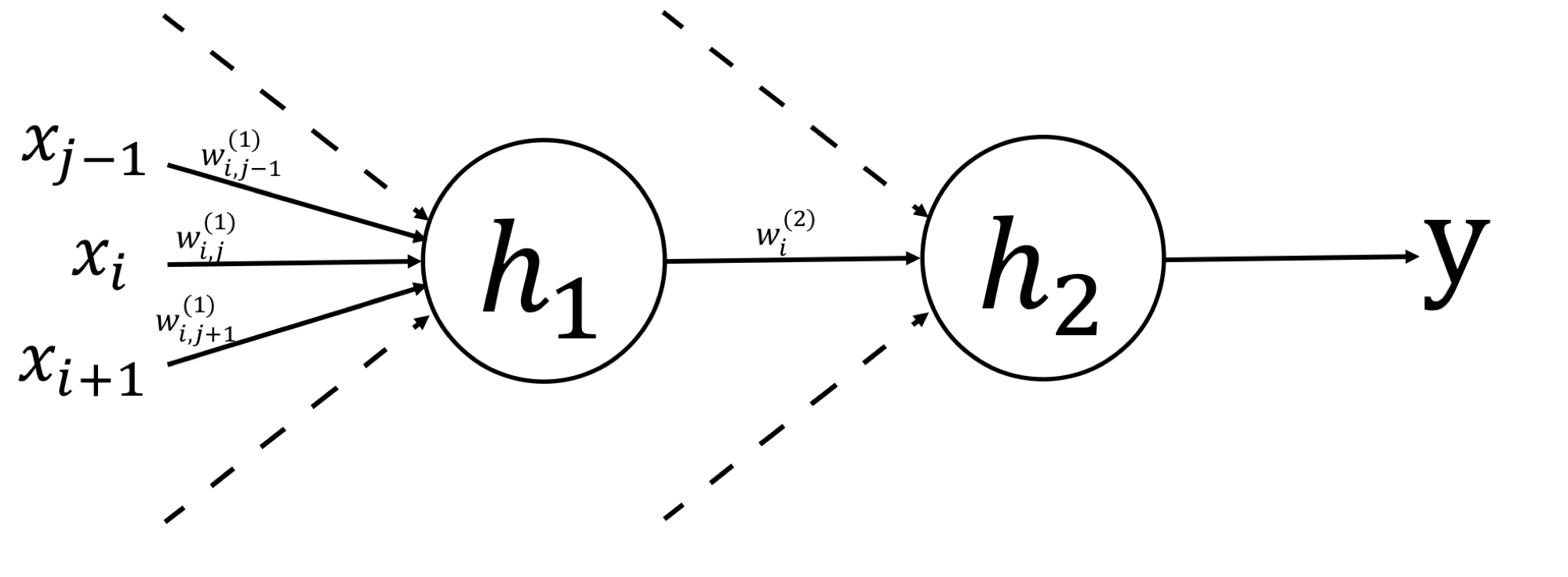

Why multi Layers ??¶

$$ \begin{aligned} &\text{single :} &y&=f\left(\sum_i w_i\underbrace{\phi_i(\mathbf{x})}\right)\\ &\text{multi :} &y&=h_2\left(\sum_{i=0}^{m} w^{(2)}_i \underbrace{h_1\left(\sum_{j=0}^{D}w^{(1)}_{ij} x_j\right)}\right) \end{aligned} $$

By comparing the above two equations, we can see that the "fixed" basis function $\phi_i$ becomes “adaptively fluctuate”.

$$\phi_i(\mathbf{x})\rightarrow\displaystyle h_1\left(\sum_{j=0}^{D}w^{(1)}_{ij} x_j\right)$$

Therefore, it is said that "If Neural Networks have sufficient layers and neurons, they can compute any function at all."

Backpropagation

In the context of Neural Networks, "training" is "to minimize the error $E_n(\mathbf{w})$ between the output and the correct answer by changing the weight", and to achive this it is necessary to calculate $\frac{\partial E_n}{w_{ji}}$ for all $i, j$.

forward	backprop

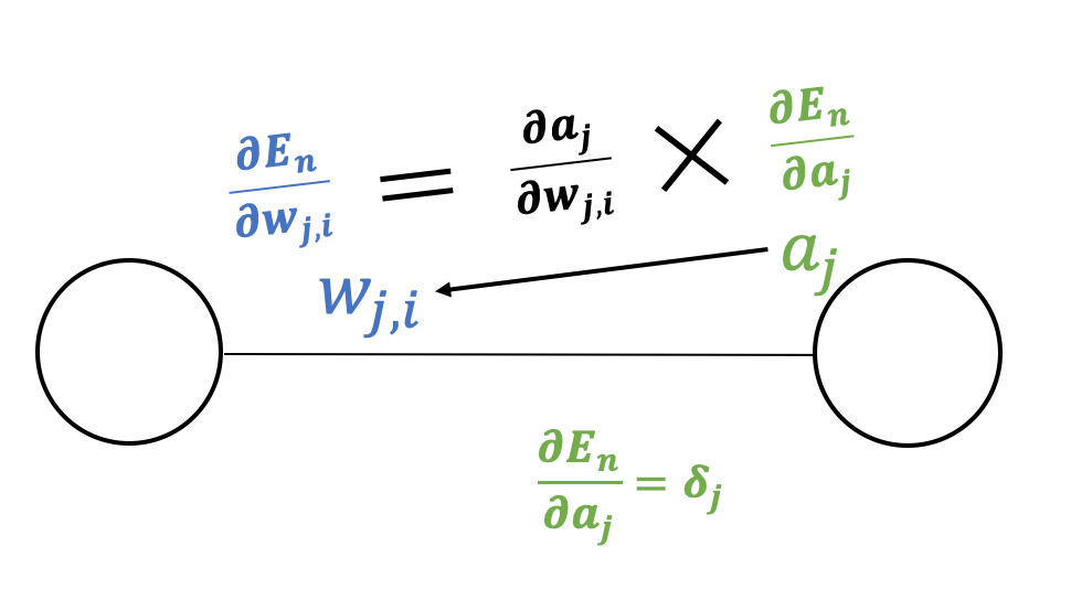As shown in the figure above, as "$E_n$ depends on $w_{ji}$ only via $a_j$", we can get the following formula.

$$ \frac{\partial E_n}{\partial w_{ji}} = \underbrace{\frac{\partial E_n}{\partial a_j}}_{\delta_j}\frac{\partial a_j}{\partial w_{ji}}$$

Likewise, as "$E_n$ depends on $a_i$ only via $a_j$ which receives the output of neuron $j$", we can get

$$ \delta_i = \frac{\partial E_n}{\partial a_i} = \sum_j \frac{\partial E_n}{\partial a_j}\frac{\partial a_j}{\partial a_i} = \sum_j\delta_j\frac{\partial a_j}{\partial a_i}$$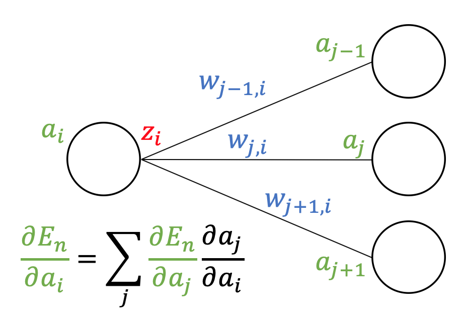

Since the formula

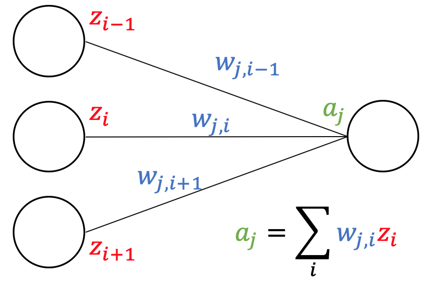
$$a_j = \sum_i w_{ji} h_i(a_i)\quad \left(\because z_i = h_i(a_i)\right)$$

holds, we can get

$$ \frac{\partial a_j}{\partial a_i} = w_{ji} h_i'(a_i)$$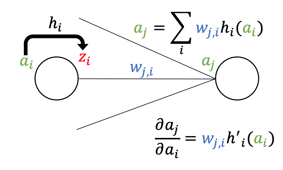

To summarize the results so far, we can derive the backpropagation formula for $\delta$

$$ \delta_i = h_i'(a_i) \sum_j w_{ji}\delta_j$$

Using the backpropagation formula, once we go back through the network from output to input, we can compute all $\frac{\partial E_n}{w_{ji}}$, and update the weights efficiently.

Example

Data¶

Model¶