Alignment
Notebook
Example Notebook: Kerasy.examples.alignment.ipynb
Why compare DNA sequences?
- To understand the function of the DNA. (The more similar the DNA sequences are the more similar the functions are.)
- To find where are the important region.
- To know the phylogenetic tree of organisms.
- To inspect where the DNA come from.
Needleman-Wunsch-Gotoh
class kerasy.Bio.alignment.NeedlemanWunshGotoh(**kwargs)
- Global Alignment: Align the entire two sequences.
- Direction: Forward
- params:
matchmismatchgap_openinggap_extension
$$
\begin{aligned}
M(i,j) &= \max
\begin{cases}
M(i-1,j-1) + s(x_i, y_j)\\
X(i-1,j-1) - s(x_i, y_j)\\
Y(i-1,j-1) - s(x_i, y_j)
\end{cases}\\
X(i,j) &= \max
\begin{cases}
M(i-1,j) - d\\
X(i-1,j) - d\\
\end{cases}\\
Y(i,j) &= \max
\begin{cases}
M(i,j-1) - d\\
Y(i,j-1) - d\\
\end{cases}\\
d &= \text{gap opening penalty}\\
e &= \text{gap extension penalty}\\
s(x_i,y_j) &=
\begin{cases}
\text{match score} & (\text{if $x_i=y_j$})\\
\text{mismatch score} & (\text{otherwise.})\\
\end{cases}
\end{aligned}
$$
Backward Needleman-Wunsh-Gotoh
class kerasy.Bio.alignment.BackwardNeedlemanWunshGotoh(**kwargs)
- Global Alignment:
- Direction: Backward
- params:
matchmismatchgap_openinggap_extension
$$
\begin{aligned}
bM(i,j) &= \max
\begin{cases}
bM(i+1,j+1) + s(x_{i+1}, y_{j+1})\\
bX(i+1,j) - d\\
bY(i,j+1) - d
\end{cases}\\
bX(i,j) &= \max
\begin{cases}
bM(i+1,j+1) + s(x_{i+1},y_{j+1})\\
bX(i+1,j) - e
\end{cases}\\
bY(i,j) &= \max
\begin{cases}
bM(i+1,j+1) - s(x_{i+1},y_{j+1})\\
Y(i,j+1) - e\\
\end{cases}\\
\end{aligned}
$$
This algorithm is for find the maximum alignment under the condition of \(x_i\) and \(y_j\) are aligned. It is given by:
$$A(i,j) = M(i,j) + bM(i,j)$$
Smith-Waterman
class kerasy.Bio.alignment.SmithWaterman(**kwargs)
- Local Alignment: Detect the most similar part of the sequences and align them.
- Direction: Forward
- params:
matchmismatchgap_openinggap_extension
$$
\begin{aligned}
M(i,j) &= \max
\begin{cases}
0\\
M(i-1,j-1) + s(x_i, y_j)\\
X(i-1,j-1) - s(x_i, y_j)\\
Y(i-1,j-1) - s(x_i, y_j)
\end{cases}\\
X(i,j) &= \max
\begin{cases}
M(i-1,j) - d\\
X(i-1,j) - d\\
\end{cases}\\
Y(i,j) &= \max
\begin{cases}
M(i,j-1) - d\\
Y(i,j-1) - d\\
\end{cases}\\
\end{aligned}
$$
Pair HMM
class kerasy.Bio.alignment.PairHMM(**kwargs)
We can interpret alignment probabilistically.
$$
\begin{aligned}
P(\pi|x,y) &= \frac{P(x,y,\pi)}{P(x,y)}\\
P(x,y) &= \sum_{\text{alignments }\pi}P(x,y,\pi)\\
P(x_i\diamondsuit y_i|x,y)
&= \frac{\sum_{\pi\in\Omega_{ij}}P(x,y,\pi)}{P(x,y)}\\
&= \frac{F^M(i,j)\cdot B^M(i,j)}{P(x,y)}
\end{aligned}
$$
| Probability | Explanation |
|---|---|
|
$$P(\pi\mid x,y)$$
|
The probability of alignment \(\pi\) is obtained given \(x_i\) and \(y_j\). |
|
$$P(x_i\diamondsuit y_i\mid x,y)$$
|
The probability of \(x_i\) and \(y_j\) are aligned. |
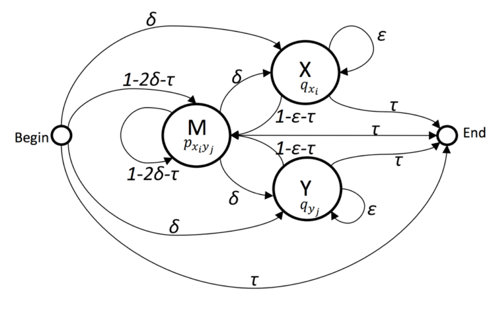
- Global Alignment
- Direction: Forward
- params:
deltaepsilontaupx_e_ypx_ne_yqxqy
Viterbi Algorithm
$$
\begin{aligned}
V^M(i,j) &= p_{x_iy_j}\max\begin{cases}(1-2\delta-\tau)V^M(i-1,j-1)\\(1-\varepsilon-\tau)V^X(i-1,j-1)\\(1-\varepsilon-\tau)V^Y(i-1,j-1)\end{cases}\\
V^X(i,j) &= q_{x_i}\max\begin{cases}\delta V^M(i-1,j)\\\varepsilon V^X(i-1,j)\end{cases}\\
V^Y(i,j) &= q_{y_j}\max\begin{cases}\delta V^M(i,j-1)\\\varepsilon V^X(i,j-1)\end{cases}\\
V^E(n,m) &= \tau\max\left(V^M(n,m),V^X(n,m),V^Y(n,m)\right)
\end{aligned}
$$
Forward Algorithm
$$
\begin{aligned}
F^M(i,j) &= p_{x_iy_j}\text{sum}\begin{cases}(1-2\delta-\tau)F^M(i-1,j-1)\\(1-\varepsilon-\tau)F^X(i-1,j-1)\\(1-\varepsilon-\tau)F^Y(i-1,j-1)\end{cases}\\
F^X(i,j) &= q_{x_i}\text{sum}\begin{cases}\delta F^M(i-1,j)\\\varepsilon F^X(i-1,j)\end{cases}\\
F^Y(i,j) &= q_{y_j}\text{sum}\begin{cases}\delta F^M(i,j-1)\\\varepsilon F^X(i,j-1)\end{cases}\\
F^E(n,m)
&= \tau\ \text{sum}\left(F^M(n,m),F^X(n,m),F^Y(n,m)\right)
\end{aligned}
$$
Backward Algorithm
$$
\begin{aligned}
B^M(i,j) &= \text{sum}\begin{cases}(1-2\delta-\tau)p_{x_iy_j}B^M(i+1,j+1)\\\delta q_{x_{i+1}}B(i+1,j)\\\delta q_{y_{j+1}}B^Y(i,j+1)\end{cases}\\
B^X(i,j) &= (1-\varepsilon-\tau)p_{x_{i+1},y_{j+1}}B^M(i+1,j+1) + \varepsilon q_{x_{i+1}}B^X(i+1,j)\\
B^Y(i,j) &= (1-\varepsilon-\tau)p_{x_{i+1},y_{j+1}}B^M(i+1,j+1) + \varepsilon q_{y_{j+1}}B^Y(i,j+1)\\
\end{aligned}
$$
Baum-Welch Algorithm
Although the ordinary Hidden Markov Models calculate the optimal parameters from the perspective of time span \(t\), PairHMM focus on the position \(u,v\) of each sequence.
Estep
$$
\begin{aligned}
\xi_{u,v}\left(i,j\right)
&=\frac{f_i\left(u,v\right)A_{ij}\phi_j\left(\diamond_1\right)b_j\left(\diamond_2,\diamond_3\right)}{\sum_{k=1}^Kf_k\left(u,v\right)b_k\left(u,v\right)}\\
\gamma_i\left(u,v\right)
&=\frac{f_i\left(u,v\right)b_j\left(u,v\right)}{\sum_{k=1}^Kf_k\left(u,v\right)b_k\left(u,v\right)}
\end{aligned}
$$
| variable | meaning |
|---|---|
| \(f_i\left(u,v\right)\) | The probability of ending up in state \(i\) after aligning the two sequences \(\mathbf{X,Y}\) up to observation \(u\) and \(v\) respectively. |
| \(A_{ij}\) | the transition probability from state \(i\) to state \(j\). |
| \(\phi_j\left(\diamond_1\right)\) | the emission probability of emitting \(\diamond_1\) in state \(j\). |
| \(b_j\left(\diamond_2,\diamond_3\right)\) | the probability of being in state \(j\), given the sequences \(\mathbf{X,Y}\) are aligned from observation \(\diamond_2+1\) and \(\diamond_3+1\) to the end of the sequences respectively. |
※ "\(\diamond_{[1,2,3]}\)" depends on the states (\(M,X,Y\)) as below:
| state\variable | \(\phi_j\left(\diamond_1\right)\) | \(b_j\left(\diamond_2,\diamond_3\right)\) |
|---|---|---|
| \(M\) | \(e\left(x_{u+1},y_{v+1}\right)\) | \(b_j\left(u+1,v+1\right)\) |
| \(X\) | \(e\left(x_{u+1}\right)\) | \(b_j\left(u+1,v\right)\) |
| \(Y\) | \(e\left(y_{v+1}\right)\) | \(b_j\left(u,v+1\right)\) |
M step
(\pi_k)
$$\pi^{\star}_i = \sum_w\gamma_i^w(0,0)$$
(A_{ij})
$$A^{\star}_{ij} = \frac{\sum_w\sum_{u=0}^{\tilde{U}}\sum_{v=0}^{\tilde{V}}\xi_{u,v}^{w}\left(i,j\right)}{\sum_w\sum_{u=0}^{\tilde{U}}\sum_{v=0}^{\tilde{V}}\sum_{j}^{K}\xi_{u,v}^{w}\left(i,j\right)}$$
| final emitting state | \(\tilde{U}\) | \(\tilde{V}\) |
|---|---|---|
| \(M\) | \(U-1\) | \(V-1\) |
| \(X\) | \(U-1\) | \(V\) |
| \(Y\) | \(U\) | \(V-1\) |
(\phi_{i}(k))
$$\phi_i\left(k\right) = \frac{\sum_w\sum_{u=0}^{U\ast1}\sum_{v=0}^{V\ast2}\gamma_i^w\left(u,v\right)}{\sum_w\sum_{u=0}^U\sum_{v=0}^V\gamma_i^w\left(u,v\right)}$$
- \(\ast1\):\(x_u=k_x\) and state \(i\) equals the state \(M\) or \(X\). (in the state \(Y\), a gap is present in observation stream \(x\) therefore \(k_x\) is not present.)
- \(\ast2\):\(y_v=k_y\) and state \(j\) equals the state \(M\) or \(Y\).
Reference