Computational Graph
A computational graph is a directed graph where
- the nodes correspond to opecodes (operations).
- the edges correspond to operands (variables).
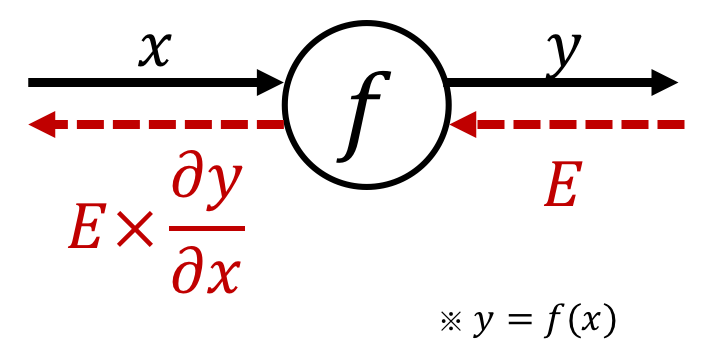
By using computational graph, it is possible to obtain the final calculation result by propagating the local calculation, which simplifies the problem.
Especially in the backpropagation method, the "chain rule" is exactly the localization of the calculation, so it has good compatibility.
Chain rule vs. Computational graph
$$\text{ex.)}\quad z=(x+y)^2$$| Chain rule | Computational graph |
|---|---|
| $$\begin{cases}z = t^2\\t = x+y\end{cases}\\ \Longrightarrow\frac{\partial z}{\partial x} = \frac{\partial z}{\partial t} \times \frac{\partial t}{\partial x}$$ | 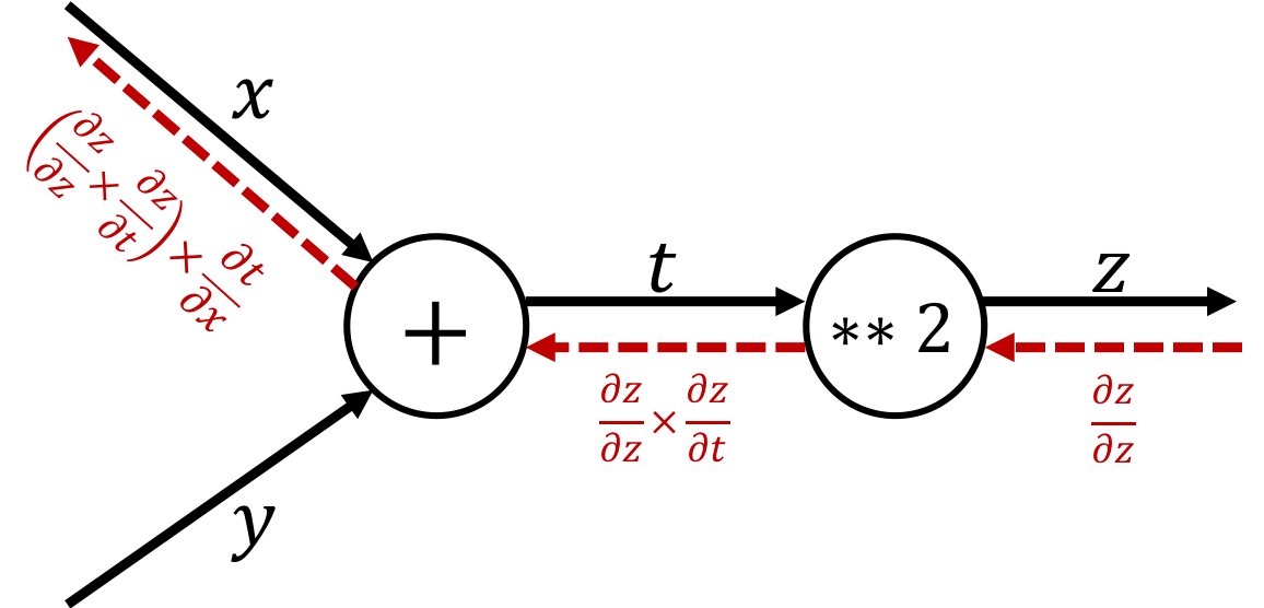 |
Add
$$\text{ex.)}\quad z=x+y$$The derivative can be calculated as
$$ \begin{cases} \begin{aligned} \frac{\partial z}{\partial x} = 1\\ \frac{\partial z}{\partial y} = 1\\ \end{aligned} \end{cases} $$Therefore, the backpropagation of the Add node is expressed as follows:
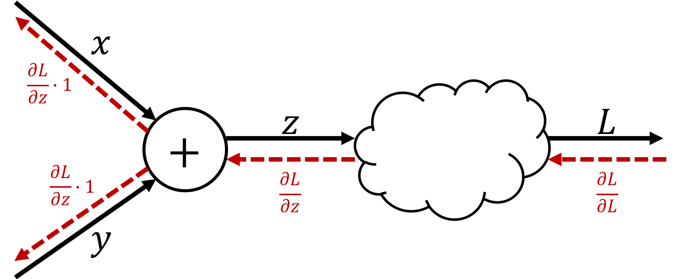
※ Just pass the differential value transmitted from the upstream to the downstream.
Mul
$$\text{ex.)}\quad z=xy$$The derivative can be calculated as
$$ \begin{cases} \begin{aligned} \frac{\partial z}{\partial x} = y\\ \frac{\partial z}{\partial y} = x\\ \end{aligned} \end{cases} $$Therefore, the backpropagation of the Mul node is expressed as follows:
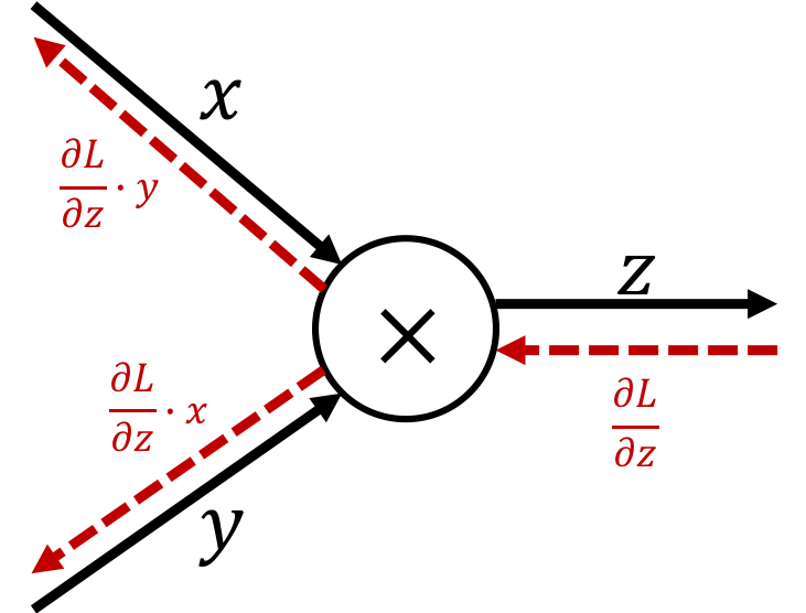
※ Multiply the "turned over value" of the input signal.
Inverse
$$\text{ex.)}\quad y=\frac{1}{x}$$The derivative can be calculated as
$$ \frac{\partial y}{\partial x} = -\frac{1}{x^2} = -y^2 $$Therefore, the backpropagation of the Inverse node is expressed as follows:
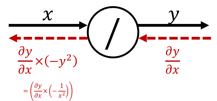
※ Multiply the minus square of "the output of forward propagation".
exp
$$\text{ex.)}\quad y=\exp(x)$$The derivative can be calculated as
$$ \frac{\partial y}{\partial x} = \exp\left(x\right) = y $$Therefore, the backpropagation of the exp node is expressed as follows:
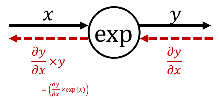
※ Multiply the minus square of "the output of forward propagation".
Connecting nodes
By connecting the above four nodes, we can easily calculate the backpropagation of Softmax and Cross Entropy Error
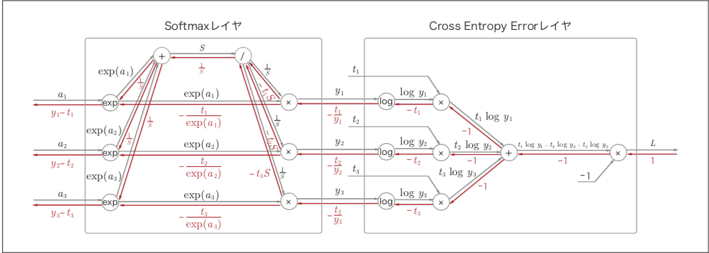
Supplementary explanation
The backpropagation of the Softmax can be expressed as follows.
$$ \begin{cases} \begin{aligned} &\sum_i\left(\underbrace{\underbrace{-\frac{t_i}{y_i}\times\exp(a_i)}_{-t_iS}\times\left(-\frac{1}{S^2}\right)}_{\frac{t_i}{S}}\right) \times \exp(a_i) = y_i\left(\because\sum_it_i=1\right)\\ &\underbrace{-\frac{t_i}{y_i}\times\frac{1}{S}}_{-\frac{t_i}{\exp(a_i)}}\times \exp(a_i) = -t_i \end{aligned} \end{cases} $$dot
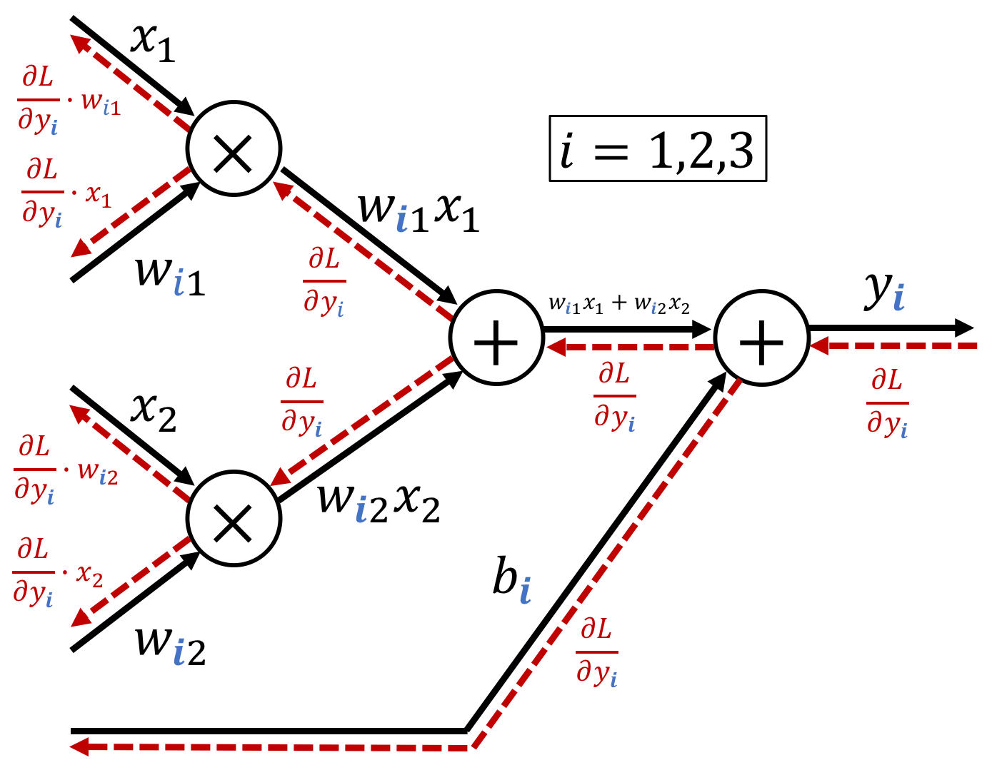
$$\text{ex.)}\quad \mathbf{Y} = \mathbf{X}\cdot\mathbf{W} + \mathbf{B}$$The derivative can be calculated as
$$ \begin{cases} \begin{aligned} \frac{\partial L}{\partial \mathbf{X}} = \frac{\partial L}{\partial \mathbf{X}}\cdot \mathbf{W}^T\\ \frac{\partial L}{\partial \mathbf{W}} = \mathbf{X}^T\cdot\frac{\partial L}{\partial \mathbf{Y}}\\ \end{aligned} \end{cases} $$Therefore, the backpropagation of the dot node is expressed as follows:
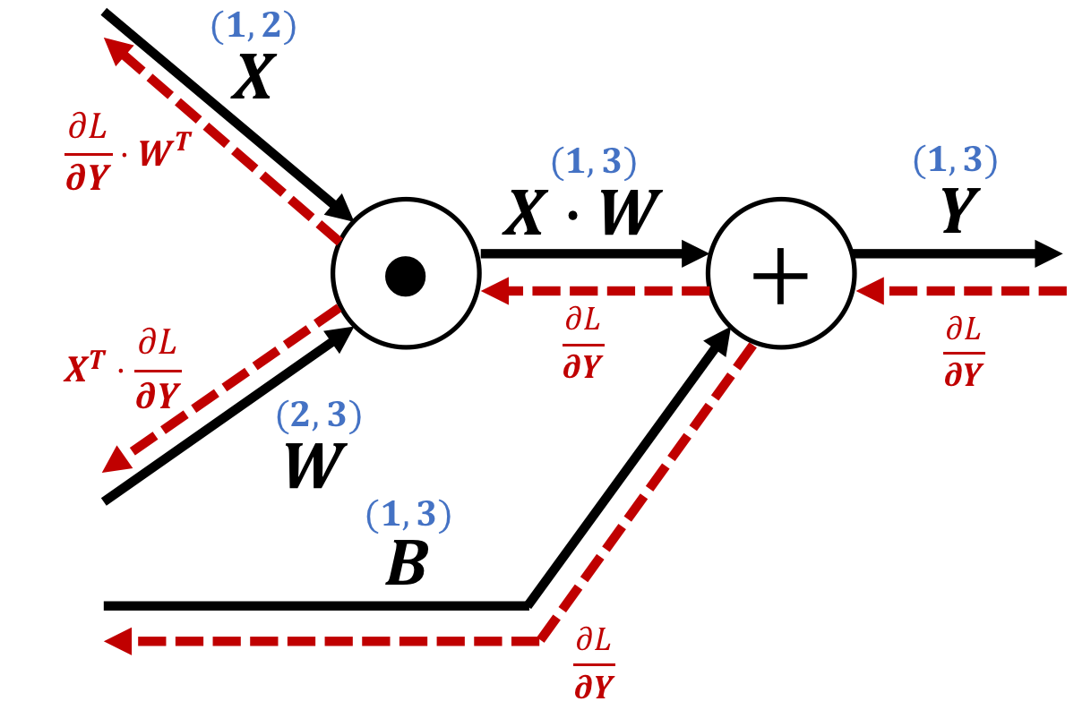
※ You can easily understand the content of the figure above by decomposing a matrix calculation into its elements and using a computational graphs in smaller units.
Implementation
Add
class Add:
    def __init__(self):
        pass

    def forward(self, x, y):
        out = x+y
        return out

    def backward(self, dout):
        dx = dout * 1
        dy = dout * 1

        return dx, dy
Mul
class Mul:
    def __init__(self):
        self.x = None
        self.y = None

    def forward(self, x, y):
        self.x = x
        self.y = y
        out = x * y

        return out

    def backward(self, dout):
        dx = dout * self.y
        dy = dout * self.x

        return dx, dy
Inverse
class Inverse:
    def __init__(self):
        self.out = None

    def forward(self, x):
        out = 1/x
        self.out = out

        return out

    def backward(self, dout):
        dx = dout * (-self.out**2)

        return dx
exp
class Exp:
    def __init__(self):
        self.out = None

    def forward(self, x):
        out = np.exp(x)
        self.out = out

        return out

    def backward(self, dout):
        dx = dout * self.out

        return dx
dot
class DotLayer:
    def __init__(self):
        self.X = None
        self.W = None

    def forward(self, X, W):
        """
        @param X   : shape=(1,a)
        @param W   : shape=(a,b)
        @return out: shape=(1,b)
        """
        self.X = X
        self.W = W
        out = np.dot(X, W) # shape=(1,b)

        return out

    def backward(self, dout):
        """
        @param dout: shape=(1,b)
        @return dX : shape=(1,a)
        @return dW : shape=(a,b)
        """
        dX = np.dot(dout, self.W.T)
        dW = np.dot(self.X.T, dout)

        return dX,dW
Reference