シミュレーション実習¶

Day.5: 生化学反応系で見られる双安定性と振動現象（力学系の基礎）

担当：黒田研究室
実習のwiki：Slides and programs

おことわり。

このノートは、はやとちって先に終わらせてしまった去年（2018）のDay5の内容となっています。色々なモデルのシミュレーションができた上、線形安定性解析について再び一から学ぶことのできる充実したスライドだったので、やって良かったと思います。

概要¶

目的：「何故ヒステリシスが起きるのか？」を力学系の道具を使って説明する。

ヒステリシスとは
双安定性
振動現象

Sel'kov model

発展課題（双安定性）
発展課題（振動）
- FitzHugh-Nagumo model
- Repressilator model
発展課題（おまけ）

1. ヒステリシスとは

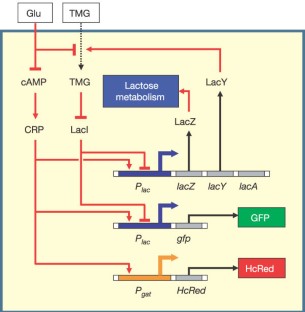
まず、「ヒステリシス（履歴依存性）が何か？」、「ヒステリンシスが生じるために必要な要素は何か？」を学ぶために、大腸菌lacオペロンの双安定性を以下のようにモデル化し、シミュレーションを行うことでヒステリンシスを再現する。

論文のモデル	簡略化したモデル

数式で書くと、以下のようになる。

$$\begin{aligned} \frac{\mathrm{d} x}{\mathrm{d} t} &=-x+\alpha X_{o u t}+\beta y \\ \frac{\mathrm{d} y}{\mathrm{d} t} &=\frac{x^{2}}{\rho+x^{2}}-y \end{aligned}$$

Variable/Constant	Meaning
$x$	細胞内TMG濃度
$y$	LacY-GFP濃度
$X_{out}$	細胞外TMG濃度
$\alpha,\beta$	Rate constants
$\rho$	Tightness of LacⅠ repression

In [1]:

import numpy as np
import matplotlib.pyplot as plt

課題1：まずはOzbudak modelを動かそう¶

In [2]:

def Ozbudak_ODE(x,y,alpha=0.1,beta=10,rho=25,x_out=5,hill=2,dt=0.01):
    dx = (-x + alpha*x_out + beta*y) * dt
    dy = (x**hill/(rho+x**hill) - y) * dt
    return x+dx,y+dy

In [3]:

def Ozbudak_model(dt=0.01, min_t=0, max_t=30,
                  alpha=0.1, beta=10, rho=25, x_out=5, hill=2, wash=None,
                  x=0,y=0,):
    max_t+=dt
    time = np.arange(min_t,max_t,dt) 
    Xs = np.zeros(len(time))
    Ys = np.zeros(len(time))
    Xouts = np.zeros(len(time))
    for i,t in enumerate(time):
        x,y = Ozbudak_ODE(x,y,alpha,beta,rho,x_out,hill,dt)
        if wash and wash/dt==i: x_out=0
        Xs[i]=x; Ys[i]=y; Xouts[i]=x_out
    if wash: return time,Xs,Ys,Xouts
    return time,Xs,Ys

In [4]:

time, Xs, Ys = Ozbudak_model(max_t=30, wash=False)

In [5]:

plt.plot(time, Xs, color="blue", label="$x(\text{TMG_{in}})$")
plt.plot(time, Ys, color="red",  label="$y(\text{LacY-GFP})$")
plt.title("simulation result")
plt.xlabel("time")
plt.ylabel("Dimensionless concentration")
plt.legend()
plt.show()

課題2：Ozbudak modelがヒステリシス（履歴依存性）を示すことを確認する¶

※ 実験的な操作として、培地から集菌してwashすることに対応

In [6]:

initial_Xouts = [i for i in range(1,11)]

In [7]:

fig = plt.figure(figsize=(16,4))
ax1=fig.add_subplot(1,2,1); ax1.set_xlabel("time"); ax1.set_ylabel("$\mathrm{X_{out}}$")
ax2=fig.add_subplot(1,2,2); ax2.set_xlabel("time"); ax2.set_ylabel("$y(\text{LacY-GFP})$")
cmap = plt.get_cmap("tab10")

for i,xout in enumerate(initial_Xouts):
    time,Xs,Ys,Xouts = Ozbudak_model(max_t=120, x_out=xout, wash=60)
    ax1.plot(time, Xouts, color=cmap(i))
    ax2.plot(time, Ys, color=cmap(i))

plt.show()

上の図から、$\mathrm{X_{out}}$ の初期値によってヒステリンシスが生じない場合（$\mathrm{X_{out}}\leq7$）と生じる場合（$\mathrm{X_{out}}\geq8$）があることがわかる。

In [8]:

fig = plt.figure(figsize=(16,4))

for i,xout in enumerate([5,10]):
    time,Xs,Ys,Xouts = Ozbudak_model(max_t=120, x_out=xout, wash=60)
    
    ax=fig.add_subplot(1,2,i+1)
    ax.set_xlabel("time")
    ax.set_ylabel("$y(\text{LacY-GFP})$")
    ax.set_title("$\mathrm{X_{out}}(t=0)=" + "{}$".format(xout))
    ax.plot(time, Ys, color="blue")
plt.show()

課題3：ヒステリシスが起きるTMGの濃度を図示する¶

時系列を dose response curve に描き直す

X軸：$\mathrm{TMG_{out}}$
Y軸：$\mathrm{LacY-GFP}$ の最終値

実験的な操作としては以下

$\mathrm{TMG}=\mathrm{X\ \mu M}$ で培養
集菌（$x$ がリセットされ、$y$ は保存される。）
$\mathrm{TMG}=\mathrm{\left(X\pm\Delta X\right)\ \mu M}$ で培養
以降上記操作の繰り返し

In [9]:

def RepeatCulture(ax,step,max_x_out,title="",dt=0.01,min_t=0,max_t=30,
                  alpha=0.1,beta=10,rho=25,x_out=5,hill=2,wash=None,
                  x=0,y=0,):
    x_out=0
    Ys=[0]
    
    label="Priod of increase"
    while x_out<=max_x_out:
        if wash:
            _,_,Ys,_ = Ozbudak_model(dt,min_t,max_t,alpha,beta,rho,x_out,hill,wash,x,y=Ys[-1])
        else:
            _,_,Ys = Ozbudak_model(dt,min_t,max_t,alpha,beta,rho,x_out,hill,wash,x,y=Ys[-1])
            
        ax.scatter(x_out,Ys[-1], marker="o", color='white', edgecolors='black', s=100, label=label)
        x_out+=step
        label=None
        
    label="Period of decrease"
    while x_out>=0:
        if wash:
            _,_,Ys,_ = Ozbudak_model(dt,min_t,max_t,alpha,beta,rho,x_out,hill,wash,x,y=Ys[-1])
        else:
            _,_,Ys = Ozbudak_model(dt,min_t,max_t,alpha,beta,rho,x_out,hill,wash,x,y=Ys[-1])
            
        ax.scatter(x_out,Ys[-1], marker="+", color="red", s=100, label=label)
        x_out-=step
        label=None
    ax.set_title("simulation result: " + title)    
    ax.set_xlabel("$\mathrm{X_{out}}(\mathrm{TMG_{out}})$")
    ax.set_ylabel("$y(\mathrm{LacY-GFP_{end}})$")
    ax.legend()
    return ax

In [10]:

fig, axes = plt.subplots()
axes = RepeatCulture(axes, step=1, max_x_out=20)
plt.show()

課題4：ポジティブ・フィードバックを切るとヒステリシスは起きなくなる¶

ポジティブ・フィードバックを遮断する（弱める：$\beta = 10\rightarrow5$）

In [11]:

fig, axes = plt.subplots()
axes = RepeatCulture(axes, step=1, max_x_out=30, title="(beta=5)", beta=5)
plt.show()

どちらも同じS字カーブを描く。

課題5：協調作用がなくなるとヒステリシスは起きなくなる¶

協調作用がない $\Leftrightarrow$ Hill係数が $1$

In [12]:

fig, axes = plt.subplots()
axes = RepeatCulture(axes, step=5, max_x_out=130, title="Hill=1", hill=1)
plt.show()

結論¶

In [13]:

fig = plt.figure(figsize=(16,4))
ax = fig.add_subplot(1,3,1); ax=RepeatCulture(ax,step=1,max_x_out=30,title="without Positive feedback",beta=5)
ax = fig.add_subplot(1,3,2); ax=RepeatCulture(ax,step=1,max_x_out=20,title="with both")
ax = fig.add_subplot(1,3,3); ax=RepeatCulture(ax,step=5,max_x_out=130,title="without Cooperative action",hill=1)
plt.tight_layout()
plt.show()

ヒステリシスには次の2因子が必要である

ポジティブ・フィードバック

協調作用

→じゃあ、なんでこれらの要素が必要なのか？（こっから本題！！）

以下の力学系の道具を使って説明していく。

相平面
ヌルクライン
固定点
ベクトル場
ヤコビ行列と固有値・固有ベクトル

2. 双安定性

2.1. 相平面

時間変化する2変数を縦軸・横軸にとった平面
ここでは、$x(\mathrm{TMG_{out}})-y(\mathrm{LacY-GFP_{end}})$ 平面のこと。

2.2 ヌルクライン

$dx/dt=0,dy/dt=0$ となる点の集まりからなる曲線
ヌルクラインの交点は「固定点」とも呼ばれる。（※分野によっては平衡点とも呼ぶ）

$$\begin{aligned} \frac{\mathrm{d} x}{\mathrm{d} t} &=-x+\alpha X_{o u t}+\beta y=0 &\therefore\ y &=\frac{1}{\beta}\left(x-\alpha X_{o u t}\right)\\ \frac{\mathrm{d} y}{\mathrm{d} t} &=\frac{x^{2}}{\rho+x^{2}}-y=0 &\therefore\ y &=\frac{x^{2}}{\rho+x^{2}} \end{aligned}$$

課題6：相平面とヌルクライン¶

Ozbudakモデルの解軌跡を相平面に描きなさい。
ヌルクラインの式を紙と鉛筆で求め、グラフ化しなさい。

In [14]:

def Ozbudak_nurclines(ax,
                      alpha=0.1,beta=10,rho=25,x_out=5,
                      xmin=0,xmax=10,ymin=0,ymax=0.8,
                      label=True,lwidth=1):
    nurcline1 = lambda x:(x-alpha*x_out)/beta
    nurcline2 = lambda x:x**2/(rho+x**2)
    X = np.linspace(xmin,xmax,1000)
    Y1 = np.vectorize(nurcline1)(X)
    Y2 = np.vectorize(nurcline2)(X)
    ax.plot(X,Y1,label="nurcline1" if label else None, linewidth=lwidth, color="red")
    ax.plot(X,Y2,label="nurcline2" if label else None, linewidth=lwidth, color="blue")
    ax.set_xlim(xmin,xmax)
    ax.set_ylim(ymin,ymax)
    return ax

In [15]:

X_outs = [2,5,10]

In [16]:

fig = plt.figure(figsize=(16,8))
x_int=6 # 初期パラメータ
for i,x_out in enumerate(X_outs):
    time, Xs, Ys = Ozbudak_model(max_t=30, wash=False, x_out=x_out, x=x_int)
    ax=fig.add_subplot(2,3,i+1)
    ax.plot(Xs,Ys,color="black")
    ax.scatter(Xs[0],Ys[0],marker="o",color="white",edgecolors='black',s=100,label="start")
    ax.scatter(Xs[-1],Ys[-1],marker="o",color="black",s=100,label="end")
    ax = Ozbudak_nurclines(ax,x_out=x_out)
    ax.set_title("Phase plane: $\mathrm{X_{out}}=" + "{}$".format(x_out))
    ax.set_xlabel("$\mathrm{X_{out}}(\mathrm{TMG_{out}})$")
    ax.set_ylabel("$y(\mathrm{LacY-GFP_{end}})$")
    ax.legend()
    
    ax=fig.add_subplot(2,3,i+4)
    ax.plot(time,Xs,color="blue",label="$x(\text{TMG_{in}})$")
    ax.plot(time,Ys,color="red", label="$y(\text{LacY-GFP})$")
    ax.set_title("Time series: $\mathrm{X_{out}}=" + "{}$".format(x_out))
    ax.set_xlabel("time")
    ax.set_ylabel("Dimensionless concentration")
    ax.legend()
    
plt.tight_layout()
plt.show()

2.3. 固定点

「固定点」とは、定常状態のこと。
ヌルクラインの交点（固定点）では、$\mathrm{TMG_{out}},\mathrm{LacY-GFP_{end}}$ がともに変化しないので、定常状態となる。
「時系列が定常状態に達した」$\Longleftrightarrow$「相平面上では解軌跡が固定点に達した」

課題7：固定点の予測¶

$\mathrm{X_{out}}=5$ において、様々な初期値からスタートし、どの固定点に収束するかを予測せよ

In [17]:

# 固定点
fixed_points_x_out_5 = np.array([
    [0.683,0.0183],
    [2.500,0.2000],
    [7.317,0.6817]
])

In [18]:

colors =  np.array(["green","blue","red"])

各点でどの固定点に収束するかをプロット¶

In [19]:

def plot_where2fix(fixed_points,colors,x_out=5,max_t=50,
                   xmin=0,xmax=10,xspan=0.5,
                   ymin=0,ymax=1, yspan=0.05):
    
    fig = plt.figure(figsize=(16,6))
    
    ax1 = fig.add_subplot(1,2,1) 
    X = np.arange(xmin,xmax+xspan,xspan)
    Y = np.arange(ymin,ymax+yspan,yspan)
    Z = np.zeros((X.shape[0],Y.shape[0]),dtype=int)
    for i,x in enumerate(X):
        for j,y in enumerate(Y):
            _, Xs, Ys = Ozbudak_model(x=x,y=y,x_out=x_out,max_t=max_t)
            ax1.plot(Xs,Ys,color="black",alpha=0.5)
            fixed_p = np.array([Xs[-1],Ys[-1]])
            Z[j][i] = np.argmin(np.sum( (fixed_p-fixed_points)**2, axis=1) )
    ax1 = Ozbudak_nurclines(ax1, x_out, label=True, lwidth=3)
    ax1.legend()
    
    ax2 = fig.add_subplot(1,2,2)
    ax2 = Ozbudak_nurclines(ax2, x_out=x_out, label=None, lwidth=3)
    X_mesh,Y_mesh = np.meshgrid(X,Y)
    for i,fp in enumerate(fixed_points):
        ax2.scatter(fp[0],fp[1],marker="o",color=colors[i],s=100,label="fixed point {}".format(i+1)) 
    ax2.scatter(X_mesh,Y_mesh,c=colors[Z].ravel(),s=10,marker="s",label="initial points") 
    
    plt.tight_layout()
    plt.show()

In [20]:

plot_where2fix(fixed_points_x_out_5,colors)

双安定まとめ

Ozbudakモデルはヒステリシスを再現する

大腸菌は糖の濃度を記憶する

ヒステリシスには次の2つの要素が必要である

ポジティブ・フィードバック
協調作用

ヒステリシスが起きる理由は力学系の言葉で説明できる

相平面、ヌルクライン、固定点

3. 振動現象

生体内での振動現象¶

起源：細胞内の生化学反応・遺伝子発現の振動

例）

心拍
血糖値
細胞分裂
概日リズム
etc...

これらの現象を観察することで、様々なモデルが提案されている。

Name	由来
Sel'kov	解糖系
FitzHugh-Nagumo	神経発火
Repressilator	合成生物学

3.1 Sel'kov モデル

課題1-1：シミュレーションで振動を確認しよう¶

In [21]:

def selkov_ODE(x,y,a=0.06,b=0.6,dt=0.01,F6Pdgree=2,isPFK=True):
    if isPFK:        
        dx = ((a*y+x**F6Pdgree*y) - x) * dt
        dy = (b - (a*y+x**F6Pdgree*y)) * dt
    else:
        dx = ((x**F6Pdgree*y) - x) * dt
        dy = (b - (+x**F6Pdgree*y)) * dt        
    return x+dx,y+dy

In [22]:

def selkov_model(dt=0.01, min_t=0, max_t=100,
                 a=0.06, b=0.6,F6Pdgree=2,isPFK=True,
                 x=1,y=1):
    max_t+=dt
    time = np.arange(min_t,max_t,dt) 
    Xs = np.zeros(len(time))
    Ys = np.zeros(len(time))
    for i,t in enumerate(time):
        x,y = selkov_ODE(x,y,a,b,dt,F6Pdgree,isPFK)
        Xs[i]=x; Ys[i]=y;
    return time,Xs,Ys

In [23]:

fig = plt.figure(figsize=(16,4))

time,Xs,Ys = selkov_model()
xlims = [(0,100),(0,20)]

for i,xlim in enumerate(xlims):
    xmin,xmax=xlim
    ax=fig.add_subplot(1,2,i+1)
    ax.plot(time,Xs,color="red",label="ADP")
    ax.plot(time,Ys,color="blue",label="F6P")
    ax.set_title("simulation result")
    ax.set_xlabel("time")
    ax.set_ylabel("Dimensionless concentration")
    ax.set_xlim(xmin,xmax)
    ax.legend()
plt.show()

入力（定数）によってF6Pが溜まる。ADPは有限の値を維持。
F6Pが大きくなると、ADPが増え、F6Pが減少する（時間遅れのNFB）

課題1-2：$x-y$ 平面上で解軌道を描く¶

相平面上での解軌道とヌルクラインも描け。

In [24]:

def selkov_nurclines(ax,
                     xmin=0,xmax=2.5,ymin=0,ymax=3,
                     a=0.06, b=0.6, F6Pdgree=2, isPFK=True,
                     label=True,lwidth=1,colors=["red","pink"]):
    if isPFK:
        nurcline1 = lambda x:x/(a+x**F6Pdgree)
        nurcline2 = lambda x:b/(a+x**F6Pdgree)
    else:
        nurcline1 = lambda x:1/(x**(F6Pdgree-1))
        nurcline2 = lambda x:b/(x**F6Pdgree)        
    X = np.linspace(xmin,xmax,1000)
    Y1 = np.vectorize(nurcline1)(X)
    Y2 = np.vectorize(nurcline2)(X)
    ax.plot(X,Y1,label="nurcline1" if label else None, linewidth=lwidth, color=colors[0])
    ax.plot(X,Y2,label="nurcline2" if label else None, linewidth=lwidth, color=colors[1])
    ax.set_xlim(xmin,xmax)
    ax.set_ylim(ymin,ymax)
    return ax

In [25]:

fig, axes = plt.subplots()
time,Xs,Ys = selkov_model()
axes.plot(Xs,Ys,color="blue")
axes = selkov_nurclines(axes,lwidth=3)
axes.legend()
axes.set_title("simulation result")
axes.set_xlabel("ADP")
axes.set_ylabel("F6P")
plt.show()

課題1-3：入力が大きくなる or 小さくなるとどうなるか¶

入力（定数）$b$ の大きさを変化させる。

In [26]:

fig = plt.figure(figsize=(16,8))

bs=[0.1,0.3,0.5,0.7,0.9,1.1]
pos=[1,3,5,2,4,6]

for p,b in zip(pos,bs):
    time,Xs,Ys = selkov_model(b=b,max_t=100)
    ax=fig.add_subplot(3,2,p)
    ax.plot(time,Xs,color="red",label="ADP")
    ax.plot(time,Ys,color="blue",label="F6P")
    ax.set_title("simulation result: b={}".format(b))
    ax.set_ylim(0,3)
    ax.legend()
plt.tight_layout()
plt.show()

左側（$b$ 小）の間は「入力の増加」 → 「振幅：増加 / 振動数：増加」
右側（$b$ 大）の間は「入力の増加」 → 「振幅：減少 / 振動数：増加」

課題1-4/1-5：Sel'kovモデルの振動解に必要なパラメータを調べる¶

ADPによるF6Pの生成に置いてF6Pの次数（協調性）が変わる
PFKによる基礎生成が変わる（$a$ の値を変える）

時に振動が起こるか、また入力依存性を調べる。

ADPによるF6Pの生成におけるF6Pの次数（協調性）¶

F6P（$x$）の次数が $1$ の時¶

In [27]:

fig = plt.figure(figsize=(8,8))
axR = plt.subplot2grid((6,2), (0,1), rowspan=6)
axR.set_title("simulation result: F6Pdgree=1")
axR.set_xlabel("ADP")
axR.set_ylabel("F6P")

bs=[0.1,0.3,0.5,0.7,0.9,1.1]
for i,b in enumerate(bs):
    time,Xs,Ys = selkov_model(b=b,max_t=100,F6Pdgree=1)
    axR.plot(Xs,Ys,label="b={}".format(b))
    ax = plt.subplot2grid((6,2), (i,0))
    ax.plot(time,Xs,color="red",label="ADP")
    ax.plot(time,Ys,color="blue",label="F6P")
    ax.set_title("simulation result: b={}".format(b))
    ax.set_ylim(0,1.5)
    ax.legend()
    
axR.legend()
plt.tight_layout()
plt.show()

F6P（$x$）の次数が $3$ の時¶

In [28]:

fig = plt.figure(figsize=(8,8))
axR = plt.subplot2grid((6,2), (0,1), rowspan=6)
axR.set_title("simulation result: F6Pdgree=3")
axR.set_xlabel("ADP")
axR.set_ylabel("F6P")

bs=[0.1,0.3,0.5,0.7,0.9,1.1]
for i,b in enumerate(bs):
    time,Xs,Ys = selkov_model(b=b,max_t=100,F6Pdgree=3)
    axR.plot(Xs,Ys,label="b={}".format(b))
    ax = plt.subplot2grid((6,2), (i,0))
    ax.plot(time,Xs,color="red",label="ADP")
    ax.plot(time,Ys,color="blue",label="F6P")
    ax.set_title("simulation result: b={}".format(b))
    ax.set_ylim(0,6)
    ax.legend()
    
axR.legend()
plt.tight_layout()
plt.show()

次数が $1$ の時は振動せず、$3$ の時は振動した → Sel'kovモデルの振動には、ポジティブフィードバックの協調性が必要

PFKによる基礎生成は必要か？¶

$a=0$ とする。（`isPFK=False` というパラメタを用意したが、$a=0$ と同じこと。）

In [29]:

fig, axes = plt.subplots(figsize=(7,7))

int_xs=[i for i in range(1,6)]
for x in int_xs:    
    time,Xs,Ys = selkov_model(a=0,b=0.9,y=1,x=x,isPFK=False)
    axes.plot(Xs,Ys,label="initial x: {}".format(x))
axes = selkov_nurclines(axes,xmin=1e-10,a=0,b=0.9,xmax=6,ymin=1e-2,ymax=1e3,colors=["black","black"])
axes.legend()
axes.set_title("simulation result")
axes.set_xlabel("ADP")
axes.set_ylabel("F6P")
axes.set_yscale('log')
plt.show()

PFKによる基礎生成がなくなると、$(x,y) = (b, \frac{1}{b})$ が唯一の固定点となるが、$x$ が小さくなりすぎると、$v_2=v_3=0$ となり、$y$ が増加し続けてしまうこともある。その場合、振動は起こらない。

ここまでのまとめ

Ozbudakモデルのシミュレーションを行い、ポジティブフィードバックと協調性によって双安定性が現れることを確認

Sel'kovモデルのシミュレーションを行い、ポジティブ/ネガティブフィードバックによって振動が現れることを確認

フィードバックがあれば必ず双安定や振動は現れるか？　→　否。フィードバックの強さなどと密接に関係

4. 発展課題（双安定性）

この後の発展問題は、ここまで扱ってきたモデルの線形安定性解析に関する問題

4.1 固定点

固定点とは、以下の連立方程式を満たす点である。

$$ \begin{cases} dx/dt &= 0\\ dy/dt &= 0\\ \end{cases} $$

発展課題（双安定性）1-1：固定点¶

Ozbudakモデルに3つある固定点の座標を求めなさい。

In [30]:

import sympy

In [31]:

x = sympy.Symbol('x')
y = sympy.Symbol('y')

In [32]:

alpha=0.1; beta=10; rho=25; x_out=5

In [33]:

ODE1 = -x + alpha*x_out + beta*y
ODE2 = x**2/(rho+x**2) - y

In [34]:

fig, axes = plt.subplots()
axes = Ozbudak_nurclines(axes, lwidth=2)

for i,xy in enumerate(sympy.solve([ODE1, ODE2])):
    print("[fixed point {}]  x={:.3f}, y={:.3f}".format(i+1,xy[x],xy[y]))
    axes.scatter(float(xy[x]), float(xy[y]), color=colors[i], s=100, label="fixed point {}".format(i+1))

axes.set_title('"Fixed points" and "nurclines"')
axes.set_xlabel("$\mathrm{X_{out}}(\mathrm{TMG_{out}})$")
axes.set_ylabel("$y(\mathrm{LacY-GFP_{end}})$")
axes.legend()
plt.show()

[fixed point 1]  x=0.683, y=0.018
[fixed point 2]  x=2.500, y=0.200
[fixed point 3]  x=7.317, y=0.682

4.2 ベクトル場

点 $(x,y)$ に大きさ $(\dot{x},\dot{y})$ のベクトルを描いたもの

「$(\dot{x},\dot{y})$ のベクトル」はその地点の風の強さと向きに相当

発展課題（双安定性）1-2：ベクトル場を描く¶
Ozbudakモデルのベクトル場を描きなさい。

In [35]:

def plot_vector_field(ax,ODE,x_out=0.5, xmin=0,xmax=10,xspan=0.5, ymin=0,ymax=1, yspan=0.05): x = np.arange(xmin,xmax,xspan) y = np.arange(ymin,ymax,yspan) X,Y = np.meshgrid(x,y) dX,dY = ODE(x=X,y=Y) # return X+dX, Y+dY ax.quiver(X, Y, dX-X, dY-Y) return ax

In [36]:

fig, axes = plt.subplots() axes = plot_vector_field(axes, ODE=Ozbudak_ODE) axes = Ozbudak_nurclines(axes, lwidth=2) axes.set_title("vecor field") axes.set_xlabel("$\mathrm{X_{out}}(\mathrm{TMG_{out}})$") axes.set_ylabel("$y(\mathrm{LacY-GFP_{end}})$") axes.legend() plt.show()

4.3 ヤコビ行列と固有値
ヤコビ行列とは、連立微分方程式
$$ \begin{cases} \dot{x}_{1} &=f_{1}\left(x_{1}, \cdots, x_{n}\right) \\ & \vdots \\ \dot{x}_{n} &=f_{n}\left(x_{1}, \cdots, x_{n}\right) \end{cases} $$
について、
$$ J= \left\{\begin{array}{ccc}{\frac{\partial f_{1}}{\partial x_{1}}} & {\cdots} & {\frac{\partial f_{1}}{\partial x_{n}}} \\ {\vdots} & {\ddots} & {\vdots} \\ {\frac{\partial f_{n}}{\partial x_{1}}} & {\cdots} & {\frac{\partial f_{n}}{\partial x_{n}}}\end{array}\right. $$
となる行列のこと。

※ 固有値の値によって固定点に近づくのか？振動するのか？を調べるのは、システム生物学第３回（2019/6/28）で扱ったので省略する。

※ なお、黒田研の方がここにわかりやすくまとめてくださっている。

5. 発展課題（振動）

5.1 FitzHugh-Nagumo モデル
FitzHugh-Nagumo モデルは、神経発火の（簡略化）モデルであり、 4変数で複雑であったHodgkin-Huxleyと同様の振る舞いを示す2変数モデルである。

$$ \begin{cases} \begin{aligned} \frac{dv}{dt} &= v-\frac{v^3}{3}-w+\underline{\mathrm{Input}}\\ \underline{\tau}\frac{dw}{dt} &= v-a-bw \end{aligned} \end{cases} $$

変数意味

$v$ 膜電位

$w$ 不活性化変数

発展課題（振動）2-1：シミュレーションで振動を確認¶

In [37]:

def FitzHugh_Nagumo_ODE(x,y,a=0,b=1,Input=0,tau=10,dt=0.01): dx = (x - x**3/3 - y + Input) * dt dy = ((x - a - b*y) / tau ) * dt return x+dx,y+dy

In [38]:

def FitzHugh_Nagumo_model(dt=0.01,min_t=0, max_t=200, a=0,b=1,Input=0,tau=10, x=1,y=0,): max_t+=dt time = np.arange(min_t,max_t,dt) Xs = np.zeros(len(time)) Ys = np.zeros(len(time)) for i,t in enumerate(time): x,y = FitzHugh_Nagumo_ODE(x,y,a,b,Input,tau,dt) Xs[i]=x; Ys[i]=y return time,Xs,Ys

In [39]:

def FitzHugh_Nagumo_nurclines(ax, xmin=-2,xmax=2,ymin=-2,ymax=2, a=0,b=1,Input=0,tau=10, label=True,lwidth=1,alpha=1,colors=["pink","pink"]): nurcline1 = lambda x:x-x**3/3+Input nurcline2 = lambda x:(x-a)/b X = np.linspace(xmin,xmax,1000) Y1 = np.vectorize(nurcline1)(X) Y2 = np.vectorize(nurcline2)(X) ax.plot(X,Y1,label="nurcline1" if label else None, alpha=alpha, linewidth=lwidth, color=colors[0]) ax.plot(X,Y2,label="nurcline2" if label else None, alpha=alpha, linewidth=lwidth, color=colors[1]) ax.set_xlim(xmin,xmax) ax.set_ylim(ymin,ymax) return ax

In [40]:

fig = plt.figure(figsize=(16,4)) time,Xs,Ys = FitzHugh_Nagumo_model() ax1 = fig.add_subplot(1,2,1) ax1.plot(time,Xs,color="red",label="v") ax1.plot(time,Ys,color="blue",label="w") ax1.set_title("simulation result") ax1.set_xlabel("time") ax1.set_ylabel("Dimensionless concentration") ax1.legend() ax2 = fig.add_subplot(1,2,2) ax2.plot(Xs,Ys,color="blue") ax2 = FitzHugh_Nagumo_nurclines(ax2,lwidth=3) ax2.set_title("v-w Phase plane") ax2.set_xlabel("v") ax2.set_ylabel("w") ax2.legend() plt.show()

振動し、振動解を持つことがわかる！

→パラメタ（$\mathrm{Input}$）依存性を調べる。

In [41]:

fig = plt.figure(figsize=(12,12)) axR = plt.subplot2grid((9,2), (0,1), rowspan=6) axR.set_title("simulation result: F6Pdgree=1") axR.set_xlabel("ADP") axR.set_ylabel("F6P") Inputs=[-0.4,-0.3,-0.2,-0.1,0,0.1,0.2,0.3,0.4] for i,Input in enumerate(Inputs): time,Xs,Ys = FitzHugh_Nagumo_model(Input=Input,max_t=200) axR.plot(Xs,Ys,label="Input={}".format(Input)) axR = FitzHugh_Nagumo_nurclines(axR,Input=Input,label=False,alpha=0.5,colors=["black","black"]) ax = plt.subplot2grid((9,2), (i,0)) ax.plot(time,Xs,color="red",label="v") ax.plot(time,Ys,color="blue",label="w") ax.set_title("simulation result: Input={}".format(Input)) ax.set_ylim(-2,2) ax.legend() axR.legend() plt.tight_layout() plt.show()

5.2 Repressilator モデル
Repressilator モデルは、3種類のタンパク質が各々異なるタンパク質のプロモーター領域に結合・発現を抑制するモデルである。なお、天然にはない組み合わせであり、人工的に合成されている。

$$ \begin{cases} \begin{aligned} \frac{dm_i}{dt} &= -m_i + \frac{\alpha}{1+p_j^n} + \alpha_0\\ \frac{dp_i}{dt} &= \beta\left(m_i-p_i\right)\\ \left(i,j\right) &= \left(\mathrm{TetR,LacI}\right),\left(\mathrm{LacI,\lambda cI}\right),\left(\mathrm{\lambda cI, TetR}\right) \end{aligned} \end{cases} $$

変数意味

$m_i$ mRNA

$p_i$ Protein

$-m_i$ 分解

$\frac{\alpha}{1+p^n_j}$ プロモーター領域に結合したInhibitorによる発現の阻害

$\alpha_0$ mRNAの基礎発現

$\beta m_i$ 翻訳

$-\beta p_i$ 分解

発展課題（振動）3-1：シミュレーションで振動を確認¶

In [42]:

from mpl_toolkits.mplot3d import Axes3D

In [43]:

def Repressilator_ODE(mx,my,mz,px,py,pz, alpha=100,alpha0=1,beta=5,n=2,dt=0.01): """ x：TetR y：LacI z：λcI """ dmx = (-mx + alpha/(1+py**n) + alpha0) * dt dmy = (-my + alpha/(1+pz**n) + alpha0) * dt dmz = (-mz + alpha/(1+px**n) + alpha0) * dt dpx = (beta*(mx-px)) * dt dpy = (beta*(my-py)) * dt dpz = (beta*(mz-pz)) * dt return mx+dmx,my+dmy,mz+dmz,px+dpx,py+dpy,pz+dpz

In [44]:

def Repressilator_model(dt=0.01,min_t=0,max_t=50, alpha=100,alpha0=1,beta=5,n=2, mx=4,my=5,mz=8,px=4,py=5,pz=6): time = np.arange(min_t,max_t,dt) pXs = np.zeros(len(time)) pYs = np.zeros(len(time)) pZs = np.zeros(len(time)) for i,t in enumerate(time): mx,my,mz,px,py,pz = Repressilator_ODE(mx,my,mz,px,py,pz,alpha,alpha0,beta,n,dt) pXs[i]=px; pYs[i]=py; pZs[i]=pz return time,pXs,pYs,pZs

In [45]:

fig = plt.figure(figsize=(14,4)) time,mXs,mYs,mZs = Repressilator_model() ax1 = fig.add_subplot(1,2,1) ax1.plot(time,mXs,color="blue",label="TetR") ax1.plot(time,mYs,color="green",label="LacI") ax1.plot(time,mZs,color="red",label="$\lambda$cI") ax1.set_title("simulation result") ax1.set_xlabel("time") ax1.set_ylabel("Dimensionless concentration") ax1.legend() ax2 = fig.add_subplot(1,2,2, projection='3d') ax2.view_init(azim=45) ax2.plot(mXs,mYs,mZs,color="blue") ax2.set_title("simulation dynamics") ax2.set_xlabel("TetR") ax2.set_ylabel("LacI") ax2.set_zlabel("$\lambda$cI") plt.show()

発展課題（振動）3-2：Repressilatorのパラメータ依存性¶
mRNAの基礎発現量（$\alpha_0$）を変化させる

In [46]:

fig = plt.figure(figsize=(12,8)) axR = plt.subplot2grid((7,2), (0,1), rowspan=5, projection='3d') axR.set_title("simulation result") axR.set_xlabel("TetR") axR.set_ylabel("LacI") axR.set_zlabel("$\lambda$cI") axR.view_init(azim=45) alpha0s = [10**i for i in range(-5,2)] for i,alpha0 in enumerate(alpha0s): time,mXs,mYs,mZs = Repressilator_model(alpha0=alpha0) axR.plot(mXs,mYs,mZs,label="alpha_0={}".format(alpha0)) ax = plt.subplot2grid((7,2), (i,0)) ax.plot(time,mXs,color="blue",label="TetR") ax.plot(time,mYs,color="green",label="LacI") ax.plot(time,mZs,color="red",label="$\lambda$cI") ax.set_title("simulation result: alpha0={}".format(alpha0)) ax.legend() axR.legend() plt.tight_layout() plt.show()

発展課題（振動）3-3：Repressilatorのパラメータ依存性¶
他にもパラメータ依存性を調べよ

プロモータの強さ：$\alpha$

Inhibitorの協調性：$n$

mRNAの翻訳速度及びタンパク質の分解速度 $\beta$（mRNAとタンパク質の分解速度の比）

Repressilatorの合成のために¶
パラメータ依存性を調べた研究がいくつかあり、それによって振動が起こる条件は

基礎発現（$\alpha_0$）が低く、プロモータ（$\alpha$）が強い。

mRNAとタンパク質の分解速度のバランス（$\beta$）が取れている。 

などだとわかっている。そこで、モデルを元に、振動を起こすために以下の操作が実際に行われた。

抑制時と比べ、$300\sim5000$ 倍発現するプロモータを使用。

プロテアーゼの認識部位を末端につけ、タンパク質の分解を促進 

6. 発展課題（おまけ）

6.1 Lotka-Volterra モデル
Lotka-Volterra モデル（捕食者-被捕食者モデル）は、数理生態学での振動を扱ったモデルで、元々アドリア海の魚の漁獲量が長い周期で振動する現象に対して数理的に説明したモデルである。

$$ \begin{cases} \begin{aligned} \frac{dx}{dt} &= ax - bxy\\ \frac{dy}{dt} &= cxy - dy\\ \end{aligned} \end{cases} $$

変数意味

$x$ 被捕食者

$y$ 捕食者

$-m_i$ 分解

$ax$ 一定の割合で増える

$-bxy$ 捕食者と遭遇する確率に比例して減少

$cxy$ 餌の量が多ければ増えやすい

$-dy$ 一定の割合で減少

In [47]:

def Lotka_Volterra_ODE_Naive(x,y,a=1,b=0.01,c=0.02,d=1,dt=0.01): dx = (a*x - b*x*y) * dt dy = (c*x*y - d*y) * dt return x+dx,y+dy

In [48]:

def Lotka_Volterra_model_Naive(dt=0.01,min_t=0,max_t=150, a=1,b=0.01,c=0.02,d=1, x=20,y=20): time = np.arange(min_t,max_t,dt) Xs = np.zeros(len(time)) Ys = np.zeros(len(time)) for i,t in enumerate(time): x,y = Lotka_Volterra_ODE_Naive(x,y,a,b,c,d,dt) Xs[i] = x;Ys[i] = y return time,Xs,Ys

In [49]:

fig = plt.figure(figsize=(14,4)) ax1 = fig.add_subplot(1,2,1) ax2 = fig.add_subplot(1,2,2) time,Xs,Ys = Lotka_Volterra_model_Naive() ax1.plot(Xs,Ys) ax1.set_title("Naive model simulation result") ax1.set_xlabel("Prey") ax1.set_ylabel("Predator") ax2.plot(time,Xs,color="red",label="Prey") ax2.plot(time,Ys,color="blue",label="Predator") ax2.set_title("Naive model simulation result") ax2.set_xlabel("time") ax2.set_ylabel("Dimensionless concentration") ax2.legend() plt.show()

※ 厳密には閉路モデルだが、上記の通り数値誤差の影響を受けてしまうので、初期値依存の閉路軌道にならない。そこで、許容誤差を加える。（`scipy.integrate.odeint`）

In [50]:

from scipy.integrate import odeint

In [51]:

def Lotka_Volterra_ODE(X,t,a=1,b=0.01,c=0.02,d=1,dt=0.01): dxdt = a*X[0] - b*X[0]*X[1] dydt = c*X[0]*X[1] - d*X[1] return [dxdt,dydt]

In [52]:

def Lotka_Volterra_model(dt=0.01,min_t=0,max_t=150, a=1,b=0.01,c=0.02,d=1, x=20,y=20): time = np.arange(min_t,max_t,dt) XandY = odeint(Lotka_Volterra_ODE,[x,y],time,args=(a,b,c,d,dt)) Xs = XandY[:,0] Ys = XandY[:,1] return time,Xs,Ys

In [53]:

fig = plt.figure(figsize=(12,8)) axR = plt.subplot2grid((6,2), (0,1), rowspan=6) axR.set_title("Restrict model simulation result") axR.set_xlabel("Prey") axR.set_ylabel("Predator") int_xs = [i*10 for i in range(6,17)] for i,int_x in enumerate(int_xs): time,Xs,Ys = Lotka_Volterra_model(x=int_x) axR.plot(Xs,Ys,label="initial x={}".format(int_x)) if i%2==0: ax = plt.subplot2grid((6,2), (i//2,0)) ax.plot(time,Xs,color="red",label="Prey") ax.plot(time,Ys,color="blue",label="Predator") ax.set_title("Restrict model simulation: initial x={}".format(int_x)) ax.legend() axR.legend() plt.tight_layout() plt.show()

6.2 Brusselator モデル
Brusselator モデルは、自己触媒反応の数理モデルで、実際の例としてはBelousov-Zhabotinsky(BZ)反応がある。

反応式

$$ \begin{aligned} A & \rightarrow X \\ 2 X+Y & \rightarrow 3 X \\ B+X & \rightarrow Y+D \\ X & \rightarrow E \end{aligned} $$

微分方程式

$$ \begin{aligned} \frac{\mathrm{d}[X]}{\mathrm{d} t}&=[A]+[X]^{2}[Y]-[B][X]-[X]\\ \frac{\mathrm{d}[Y]}{\mathrm{d} t}&=[B][X]-[X]^{2}[Y] \end{aligned} $$

In [54]:

def Brusselator_ODE(X=1,Y=2,A=1,B=3,dt=0.01): dX = (A + (X**2)*Y - B*X - X) * dt dY = (B*X - (X**2)*Y) * dt return X+dX,Y+dY

In [55]:

def Brusselator_model(dt=0.01,min_t=0,max_t=50, A=1,B=3,X=1,Y=2): time = np.arange(min_t,max_t,dt) Xs = np.zeros(len(time)) Ys = np.zeros(len(time)) for i,t in enumerate(time): X,Y = Brusselator_ODE(X,Y,A,B,dt) Xs[i]=X; Ys[i]=Y; return time,Xs,Ys

In [56]:

fig = plt.figure(figsize=(12,8)) axR = plt.subplot2grid((6,2), (0,1), rowspan=6) axR.set_title("simulation result") axR.set_xlabel("[X]") axR.set_ylabel("[Y]") int_Xs = [i for i in range(1,7)] for i,int_X in enumerate(int_Xs): time,Xs,Ys = Brusselator_model(X=int_X) axR.plot(Xs,Ys,label="initial [X]={}".format(int_X)) ax = plt.subplot2grid((6,2), (i,0)) ax.plot(time,Xs,color="red",label="[X]") ax.plot(time,Ys,color="blue",label="[Y]") ax.set_title("simulation result: initial [X]={}".format(int_X)) ax.legend() axR.legend() plt.tight_layout() plt.show()

6.3 More
他にも色々な振動があるので、見たい場合はRobust, Tunable Biological Oscillations from Interlinked Positive and Negative Feedback Loopsにある程度まとまっている。

また、黒田研の方が上記論文の訂正とパラメタ探索のティップスをまとめてくださっている。（ここ）感謝🙇‍♂️

# Name

1 Negative feedback and positive-plus-negative feedback cell cycle oscillators

2 Repressilator

3 Pentilator

4 Goodwin oscillator

5 Frzilator

6 Metabolator

7 Meyer and Stryer of calcium oscillations

8 van der Pol oscillators

9 FitzHugh-Nagumo oscillators

10 Cyanobacteria circadian oscillators

In [ ]:

« 生体物質化学Ⅱ 第12回

シミュレーション実習 Day5 »

シミュレーション実習¶

おことわり。

概要¶

1. ヒステリシスとは

課題1：まずはOzbudak modelを動かそう¶

課題2：Ozbudak modelがヒステリシス（履歴依存性）を示すことを確認する¶

課題3：ヒステリシスが起きるTMGの濃度を図示する¶

課題4：ポジティブ・フィードバックを切るとヒステリシスは起きなくなる¶

課題5：協調作用がなくなるとヒステリシスは起きなくなる¶

結論¶

2. 双安定性

2.1. 相平面

2.2 ヌルクライン

課題6：相平面とヌルクライン¶

2.3. 固定点

課題7：固定点の予測¶

各点でどの固定点に収束するかをプロット¶

3. 振動現象

生体内での振動現象¶

3.1 Sel'kov モデル

課題1-1：シミュレーションで振動を確認しよう¶

課題1-2：$x-y$ 平面上で解軌道を描く¶

課題1-3：入力が大きくなる or 小さくなるとどうなるか¶

課題1-4/1-5：Sel'kovモデルの振動解に必要なパラメータを調べる¶

ADPによるF6Pの生成におけるF6Pの次数（協調性）¶

F6P（$x$）の次数が $1$ の時¶

F6P（$x$）の次数が $3$ の時¶

PFKによる基礎生成は必要か？¶

4. 発展課題（双安定性）

4.1 固定点

発展課題（双安定性）1-1：固定点¶

4.2 ベクトル場

発展課題（双安定性）1-2：ベクトル場を描く¶

4.3 ヤコビ行列と固有値

5. 発展課題（振動）

5.1 FitzHugh-Nagumo モデル

発展課題（振動）2-1：シミュレーションで振動を確認¶

5.2 Repressilator モデル

発展課題（振動）3-1：シミュレーションで振動を確認¶

発展課題（振動）3-2：Repressilatorのパラメータ依存性¶

発展課題（振動）3-3：Repressilatorのパラメータ依存性¶

Repressilatorの合成のために¶

6. 発展課題（おまけ）

6.1 Lotka-Volterra モデル

6.2 Brusselator モデル

6.3 More

Table of Contents

Published

Last Updated

Category

Tags

Contact

Other contents