解答
1
$$ \begin{aligned} \frac{\partial}{\partial\mathbf{w}}L_{\rho}\left(\mathbf{w},\mathbf{z},\boldsymbol{\alpha}\right) &=\frac{\partial}{\partial\mathbf{w}}\left(\frac{1}{2}\|\mathbf{y}-\mathbf{Xw}\|_{\text{L2}}^2 + \lambda\|\mathbf{z}\|_{\text{L1}} + \boldsymbol{\alpha}^T\left(\mathbf{w}-\mathbf{z}\right) + \frac{\rho}{2}\|\mathbf{w}-\mathbf{z}\|^2_{\text{L2}}\right)\\ &=\left(-\mathbf{X}^T\mathbf{y} + \mathbf{X}^T\mathbf{Xw}\right) + \boldsymbol{\alpha} + \rho\left(\mathbf{w}-\mathbf{z}\right)\\ &= 0\\ \therefore\left(\mathbf{X}^T\mathbf{X} + \rho\mathbf{I}\right)\mathbf{w} &= \mathbf{X}^T\mathbf{y} - \boldsymbol{\alpha} + \rho\mathbf{z}\\ \therefore\underset{\mathbf{w}}{\text{argmin}}L_{\rho}\left(\mathbf{w},\mathbf{z},\boldsymbol{\alpha}\right) &= \left(\mathbf{X}^T\mathbf{X} + \rho\mathbf{I}\right)^{-1}\left(\mathbf{X}^T\mathbf{y} - \boldsymbol{\alpha} + \rho\mathbf{z}\right) \end{aligned} $$2
$z$ の正負で場合分けをすれば、
$$ \begin{aligned} \underset{z}{\text{argmin}}\left\{c|z| + \frac{1}{2}\left(z-z_0\right)^2\right\} &= \begin{cases}z_0-c & \left(z>0\right)\\z_0+c & \left(0>z\right)\\0&\left(\text{otherwise.}\right)\\\end{cases}\\ &= \begin{cases}z_0-c & \left(z_0>c\right)\\z_0+c & \left(-c>z_0\right)\\0&\left(\text{otherwise.}\right)\end{cases}\\ \end{aligned} $$3
$$ \begin{aligned} \underset{z_i}{\text{argmin}}L_{\rho}\left(\mathbf{w},\mathbf{z},\boldsymbol{\alpha}\right) &= \underset{z_i}{\text{argmin}}\left\{\lambda\|z_i\|_{\text{L1}} - \alpha_iz_i + \frac{\rho}{2}\left(-2w_iz_i + z_i^2\right)\right\}\\ &= \underset{z_i}{\text{argmin}}\left\{\lambda\|z_i\|_{\text{L1}} + \frac{\rho}{2}\left(z^2_i - 2\left(w_i + \frac{\alpha_i}{\rho}\right)z_i\right)\right\}\\ &= \underset{z_i}{\text{argmin}}\left\{\frac{\lambda}{\rho}\|z_i\|_{\text{L1}} + \frac{1}{2}\left(z_i-\left(w_i + \frac{\alpha_i}{\rho}\right)\right)^2\right\}\\ \end{aligned} $$これは、$2$ の式において
$$ \begin{cases} \begin{aligned} c&\longrightarrow\frac{\lambda}{\rho}\\ z_0&\longrightarrow w_i + \frac{\alpha_i}{\rho} \end{aligned} \end{cases} $$とした場合に対応する。以上より、
$$\underset{\mathbf{z}}{\text{argmin}}L_{\rho}\left(\mathbf{w},\mathbf{z},\boldsymbol{\alpha}\right) = \text{prox}_{\frac{\lambda}{\rho}|\ast|}\left(w_i + \frac{\alpha_i}{\rho}\right)$$ここでは、「L1正則化項の下での線形回帰問題」 を考えた。全体の流れは以下
- 二乗和誤差関数 $\frac{1}{2}\|\mathbf{y}-\mathbf{Xw}\|^2$ にL1正則化項を加えた誤差関数を定義する。($\lambda$ は手動で決定。)
- 解析的に最小解を求めるのが難しいので、新しい変数 $\mathbf{z}$ を代入してそれぞれ独立の変数としてみる。
- とはいえ $\mathbf{z}=\mathbf{w}$ という関係は成り立っているので、ラグランジュ乗数 $\{\alpha_i\}$ を導入して、制約条件を付け加える。 $$L\left(\mathbf{w},\mathbf{z},\boldsymbol{\alpha}\right) = \frac{1}{2}\|\mathbf{y}-\mathbf{Xw}\|_{\text{L2}}^2 + \lambda\|\mathbf{z}\|_{\text{L1}} + \boldsymbol{\alpha}^T\left(\mathbf{w}-\mathbf{z}\right)$$
- このままでも良いが、凸性を増すために、制約条件を二次の形で加える。この式を拡張ラグランジュ関数(Augmented Lagrangian)と呼ぶ。[参考:知能システム論 第3回] $$L_{\rho}\left(\mathbf{w},\mathbf{z},\boldsymbol{\alpha}\right) = \frac{1}{2}\|\mathbf{y}-\mathbf{Xw}\|_{\text{L2}}^2 + \lambda\|\mathbf{z}\|_{\text{L1}} + \boldsymbol{\alpha}^T\left(\mathbf{w}-\mathbf{z}\right) + \rho\|\mathbf{w}-\mathbf{z}\|_{\text{L2}}^2$$
- 解析的に求めることができないので、拡張ラグランジュ関数の最小化と双対変数の勾配上昇を繰り返す。
- 拡張ラグランジュ関数の最小化 $$\begin{aligned}\mathbf{w}&\longleftarrow \underset{\mathbf{w}}{\text{argmin}}L_{\rho}\left(\mathbf{w},\mathbf{z},\boldsymbol{\alpha}\right)\quad \text{with fixed $\mathbf{z},\boldsymbol{\alpha}$}\\\mathbf{z}&\longleftarrow \underset{\mathbf{z}}{\text{argmin}}L_{\rho}\left(\mathbf{w},\mathbf{z},\boldsymbol{\alpha}\right)\quad \text{with fixed $\mathbf{w},\boldsymbol{\alpha}$}\\\end{aligned}$$
- 双対変数の勾配上昇 $$\boldsymbol{\alpha}\longleftarrow\boldsymbol{\alpha} + \rho\nabla\omega\left(\boldsymbol{\alpha}\right) = \boldsymbol{\alpha} + \rho\left(\mathbf{w}-\mathbf{z}\right)$$
実装
以下では、実際に「線形回帰」「L1正則化項の下での線形回帰」「L2正則化項の下での線形回帰」のそれぞれを実装し、違いや特徴を調べる。
In [1]:
import numpy as np
import matplotlib.pyplot as plt
In [2]:
from kerasy.utils.data_generator import generateSin, generateGausian
sample data
In [3]:
N = 10 # data size
xmin = 0
xmax = 1
seed = 0
In [4]:
X_test_ori = np.linspace(xmin,xmax,1000)
Y_test = np.sin(2*np.pi*X_test_ori)
In [5]:
X_train_ori,Y_train = generateSin(N, xmin=xmin, xmax=xmax, seed=seed)
_, Noise = generateGausian(N, x=X_train_ori, seed=seed)
Y_train += Noise
In [6]:
plt.scatter(X_train_ori,Y_train,edgecolors='blue',facecolor="white",label="train data")
plt.plot(X_test_ori,Y_test,color="black",label="$t=\sin(2\pi x)$")
plt.legend(), plt.grid()
plt.show()

Training
In [7]:
from kerasy.utils.preprocessing import PolynomialBaseTransformer
In [8]:
Ms = [2,4,8,16]
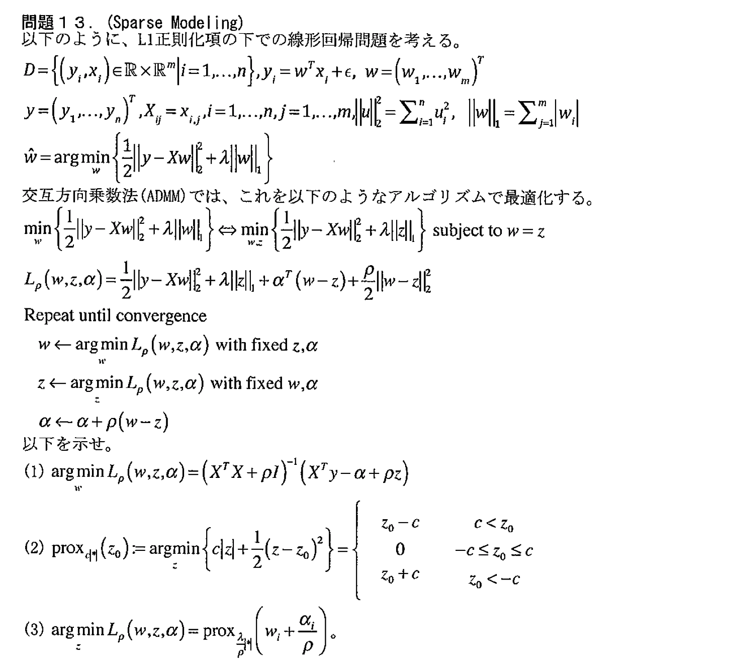
Linear Regression
In [9]:
fig=plt.figure(figsize=(16,6))

for i,M in enumerate(Ms):
    axT=fig.add_subplot(2,4,i+1)
    #=== Transform ===
    phi = PolynomialBaseTransformer(M)
    X_train = phi.transform(X_train_ori)
    X_test  = phi.transform(X_test_ori)
    #=== Training ===
    w = np.linalg.solve(X_train.T.dot(X_train), X_train.T.dot(Y_train))
    Y_pred = X_test.dot(w)
    #=== RSS ===
    RSS = np.sqrt(np.sum(np.square(X_train.dot(w)-Y_train)))

    # Plot.
    axT.plot(X_test_ori,Y_test,color="black", label="$t=\sin(2\pi x)$")
    axT.plot(X_test_ori,Y_pred,color="red", label=f"prediction ($M={M}$)")
    axT.scatter(X_train_ori,Y_train,edgecolors='blue',facecolor="white",label="train data")
    axT.set_title(f"Results (RSS=${RSS:.3f}$,M=${M}$)"), axT.set_xlabel("$x$"), axT.set_ylabel("$t$")
    axT.set_xlim(0,1), axT.set_ylim(-1.2,1.2), axT.legend()

    axB=fig.add_subplot(2,4,i+5)
    axB.barh(np.arange(len(w)),w, color="black")
    axB.set_ylim(0,max(Ms))
plt.tight_layout()
plt.savefig(f"LinearRegression_seed{seed}.png")
plt.show()

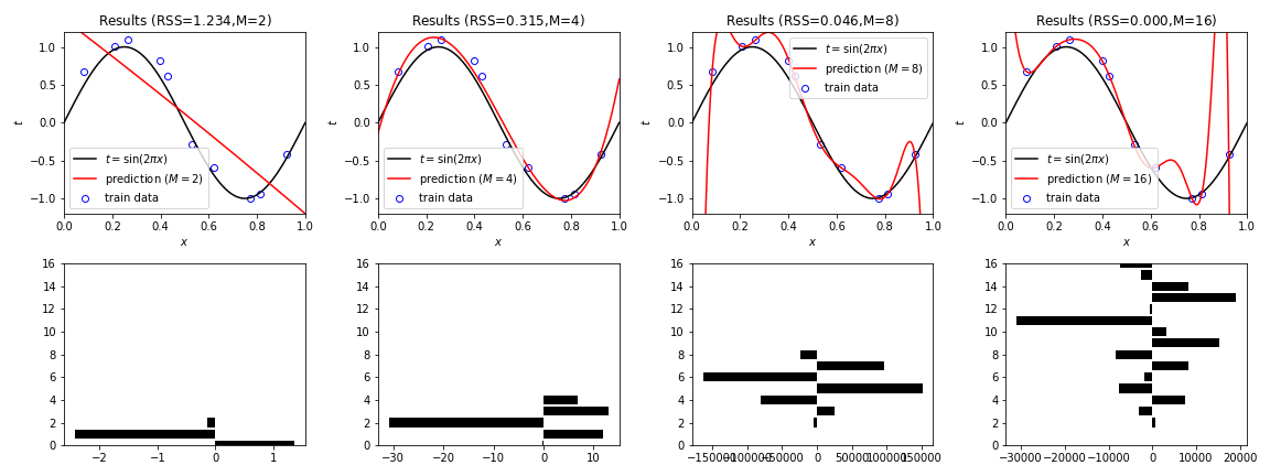
Linear Regression + L2 norm
In [10]:
lambda_ = 1e-4
In [11]:
fig=plt.figure(figsize=(16,6))

for i,M in enumerate(Ms):
    axT=fig.add_subplot(2,4,i+1)
    #=== Transform ===
    phi = PolynomialBaseTransformer(M)
    X_train = phi.transform(X_train_ori)
    X_test  = phi.transform(X_test_ori)
    #=== Training ===
    w = np.linalg.solve(lambda_*np.identity(M+1) + X_train.T.dot(X_train), X_train.T.dot(Y_train))
    Y_pred = X_test.dot(w)
    #=== RSS ===
    RSS = np.sqrt(np.sum(np.square(X_train.dot(w)-Y_train)))

    # Plot.
    axT.plot(X_test_ori,Y_test,color="black", label="$t=\sin(2\pi x)$")
    axT.plot(X_test_ori,Y_pred,color="red", label=f"prediction ($M={M}$)")
    axT.scatter(X_train_ori,Y_train,edgecolors='blue',facecolor="white",label="train data")
    axT.set_title(f"Results (RSS=${RSS:.3f}$,M=${M}$)"), axT.set_xlabel("$x$"), axT.set_ylabel("$t$")
    axT.set_xlim(0,1), axT.set_ylim(-1.2,1.2), axT.legend()

    axB=fig.add_subplot(2,4,i+5)
    axB.barh(np.arange(len(w)),w, color="black")
    axB.set_ylim(0,max(Ms))
plt.tight_layout()
plt.savefig(f"LinearRegression_L2_seed{seed}.png")
plt.show()

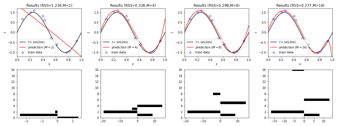
Linear Regression + L1 norm
In [12]:
lambda_ = 1e-3
rho = 1e-3
In [13]:
def prox(w,alpha,rho,lambda_):
    z0 = w + alpha/rho
    c = lambda_/rho
    return z0-c if c<z0 else z0+c if z0<-c else 0
In [14]:
fig=plt.figure(figsize=(16,6))

for i,M in enumerate(Ms):
    axT=fig.add_subplot(2,4,i+1)
    #=== Transform ===
    phi = PolynomialBaseTransformer(M)
    X_train = phi.transform(X_train_ori)
    X_test  = phi.transform(X_test_ori)
    #=== Training ===
    alpha = np.ones(shape=(M+1))
    z = np.ones(shape=(M+1))
    while True:
        w = np.linalg.solve(X_train.T.dot(X_train)+rho*np.identity(M+1), X_train.T.dot(Y_train)-alpha+rho*z)
        z = np.asarray([prox(w_,alpha_,rho,lambda_) for w_,alpha_ in zip(w,alpha)])
        alpha += rho*(w-z)
        if np.sqrt(np.sum(np.square(w-z))) < 1e-9:
            break
    Y_pred = X_test.dot(w)
    #=== RSS ===
    RSS = np.sqrt(np.sum(np.square(X_train.dot(w)-Y_train)))

    # Plot.
    axT.plot(X_test_ori,Y_test,color="black", label="$t=\sin(2\pi x)$")
    axT.plot(X_test_ori,Y_pred,color="red", label=f"prediction ($M={M}$)")
    axT.scatter(X_train_ori,Y_train,edgecolors='blue',facecolor="white",label="train data")
    axT.set_title(f"Results (RSS=${RSS:.3f}$,M=${M}$)"), axT.set_xlabel("$x$"), axT.set_ylabel("$t$")
    axT.set_xlim(0,1), axT.set_ylim(-1.2,1.2), axT.legend()

    axB=fig.add_subplot(2,4,i+5)
    axB.barh(np.arange(len(w)),w, color="black")
    axB.set_ylim(0,max(Ms))
plt.tight_layout()
plt.savefig(f"LinearRegression_L1_seed{seed}.png")
plt.show()

In [ ]: