In [1]:
import numpy as np
import matplotlib.pyplot as plt
In [2]:
import sys
sys.path.append("path/to/library") # Like "University/3A/theme/program"
Brief introduction of Differential Equations
Ordinary Differential Equations
- A fundamental tool in theoretical Science
- The differential equation gives the dependence of derivatives $$F\left[\frac{d^nx(t)}{dt^n},\cdots,\frac{dx(t)}{dt},C\right] = 0$$
- As we can calculate the whole path ways if we know the velocity($v=dx(t)/dt$), by knowing the slopes, one may trace the whole curve!!
Examples of Models and Theories
| Simple Harmonic Oscillator | Heat Equation(1-D) |
|---|---|
| An oscillator that is neither driven nor damped. | How the distribution of some quantity (such as heat) evolves over time in a solid medium |
| $$\underset{\text{Acceleration}}{\frac{d^2x(t)}{dt^2}}+\underset{\text{Returning Force}}{\omega^2x(t)} = 0$$ | $$\underset{\text{Rate of Heat}}{\frac{\partial u(x,t)}{\partial t}}+\underset{\text{Returning Force}}{\alpha\frac{\partial^2u(x,t)}{\partial x^2}} = 0$$ |
 |
 |
Implementation by Numerical Method
Euler Method
- Euler method has a relatively large error.
- There are some extensions of the Euler method(one of them are Mid-Point method.)
In [3]:
X = np.arange(-1.0,6.5,0.5)
Y = 1/6*X**3
dYdX = 1/2*X**2
In [4]:
Euler_dYdX_bigger  = (Y[2:]-Y[:-2])[2:]       # step size=1   dY/dX(t) = X(t+1)-X(t)
Euler_dYdX_smaller = (Y[1:]-Y[:-1])[2:-1]/0.5 # step size=0.5 dY/dX(t) = (X(t+0.5)-X(t))/0.5
MidPointEuler_dYdX = (Y[2:]-Y[:-2])[1:-1]     # step size=1   dY/dX(t) = X(t+0.5)-X(t-0.5)
In [5]:
def CompareNumerical(ax, X, Y, label, marker, color):
    ax.scatter(X[2:-2], Y, label=label, marker=marker, color=color)
    ax.plot(X[2:-2], Y, color=color, alpha=0.5)
    return ax
In [6]:
fig, ax = plt.subplots()
ax = CompareNumerical(ax, X, Euler_dYdX_bigger,  "Step = 1.0", "s", "b")
ax = CompareNumerical(ax, X, Euler_dYdX_smaller, "Step = 0.5", "o", "r")
ax = CompareNumerical(ax, X, MidPointEuler_dYdX, "Mid-point h=1.0", "^", "g")
ax.plot(X[2:-2], dYdX[2:-2], linestyle="--", label="Analytic", color="black")
ax.legend(), ax.grid(), ax.set_xlabel("$x$"), ax.set_ylabel("$y$")
plt.show()

The mid-point method is surprisingly good!!
Runge-Kutta Methods
- A family of implicit and explicit iterative methods.
- More: Wikipedia
Neuronal Models
To Model a Neuron...
- Neurons can be excited by current injection.
- If the membrance potential(Voltage) is larger than some thresholds, an action potential will be triggered.
- Membrance potential
- means the potential difference across the neuron membrance. → Relative
- can be controlled by concentrations of irons($\mathrm{Na}^+,\mathrm{K}^+,\mathrm{Cl}^-$)
- is maintained by their ion bumps, and at the resting state, it is around $65\mathrm{mV}$.
- sometimes across the threshold, and when it occurs, the neuron fires
- works like a capacitor with a leaky current.
Leaky Integrate-and-Fire(LIF) model

- In 1907, Lapicque proposed a simple model(which is just the time derivative of the law of capacitance ($Q=CV$).) for neurons:
$$I(t)-\frac{V_m(t) - V_{rest}}{R_m} = C_m\frac{dV_m(t)}{dt}$$
- $I$: Input current (=const.)
- $V_m$: Membrance potential
- $V_{rest}$: Resting potential of the membrance
- $R_m$: Membrane resistance (we find it is not a perfect insulator as assumed previously)
- $C_m$: Capacity of the membrance.
- When an input current is applied, the membrane voltage increases with time until it reaches a constant threshold $V_{th}$
- At the point, a delta function spike occurs and the voltage is reset to its resting potential($V_{rest}$).
- The LIF neuron fired more frequently as the input current increases.
Leak Conductance
Ion permeability at resting membrane potential, allowing a constant flow of current through the cell membrane due to channels that remain open at resting membrane potential (Ref:Encyclopedia of Neuroscience)
In [7]:
from OIST.tutorial1 import LIFsimulation, LITSpikeFrequency
In [8]:
params = {
    'V_rest': -65,
    'V_thre': -40,
    'V_reset': -70,
    'V_fire': 20,
    'C': 2e-4,
    'R': 7.5e4,
    'I': 5e-4,
    'dt': 0.1,
    'T': 100,
}
In [9]:
time, Vm = LIFsimulation(**params)
plt.plot(time, Vm, color="black")
plt.xlabel("time[ms]"), plt.ylabel("V[mV]"), plt.grid()
plt.show()

In [10]:
Is = [0.5e-3, 1e-3, 1.5e-3, 2.0e-3, 2.5e-3, 3.0e-3]
freqs = LITSpikeFrequency(Is, **params)
plt.plot(Is, freqs, color="blue"), plt.scatter(Is, freqs, color="blue", marker="s")
plt.title("How Spiking Frequency Depends on Input Current"), plt.xlabel("Input Current: I [uA]"), plt.ylabel("Spiking Frequency [Hz]"), plt.grid()
plt.show()

※ The LIF neuron fired more frequently as the input current increases.
Hodgkin-Huxley model
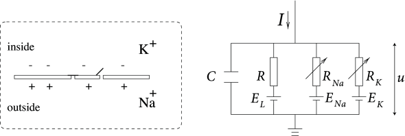
$$
I = C_m + \frac{dV_m}{dt} + g_{\mathrm{l}}\left(V_m-V_{\mathrm{l}}\right) + g_{\mathrm{K}}n^4\left(V_m-V_{\mathrm{K}}\right) + g_{\mathrm{Na}}m^3h\left(V_m-V_{\mathrm{Na}}\right)\\
\begin{cases}
\begin{aligned}
\frac{dn}{dt} &= \alpha_n(V_m)(1-n) + \beta_n(V_m)n\\
\frac{dm}{dt} &= \alpha_m(V_m)(1-m) + \beta_m(V_m)m\\
\frac{dh}{dt} &= \alpha_h(V_m)(1-h) + \beta_h(V_m)h\\
\end{aligned}
\end{cases}
$$
- Proposed by Hodgkin and Huxley in 1952 (They received the 1963 Nobel Prize in Physiology or medicin for this work.)
- Like Leaky Integrate-and-Fire(LIF) model, the input current (const.) charges up the membrance capacitor.
- Leaky conductance
- This model considers also ion currents invoving potassium ion ($\mathrm{K}^+$) and Sodium ion ($\mathrm{Na}^{+}$) induced by the potential difference.
- Sodium ion: has a reversal potential depolarizing the membrance. The conductivity is voltage-gated.
- Potassium ion: has a reversal potential hyper-polarizing the membrance. The conductivity is voltage-gated.
- The individual gates act like a first order chemical reaction with two states: $$\text{Shut}\overset{\alpha}{\underset{\beta}{\rightleftarrows}}\text{Open}$$
- Propose that
- Each $\mathrm{K}$ channel has $4$ identical activation gates.( $\mathbb{P}_{\text{open}}=n$ )
- Each $Na$ channel has $3$ avtivation gates( $\mathbb{P}_{\text{open}}=m$ ), and $1$ inactivation gate( $\mathbb{P}_{\text{open}}=h$ ).
Action Potential
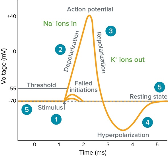
- Stimulas raises the membrane potential. (Depolarization)
- If membrance potential over the Threshold, voltage-gated sodium channels will open, and due to the sodium concentration gradient (ex > in), sodium ion flow into the cell. This process raises the membrance potential, and it gets further depolarized.
- As the membrance become **"too large"**, sodium ion channel closes, and after that (there is a delay), voltage-gated potassium channel will open.
- When the membrance potential return to the resting state, potassium channel closes, but as this response takes time, the membrance potential will be lower than the initial voltage. (Hyperpolarization)
- (※ Resting membrance potential means the equilibrium point between "electrical gradient" and "concentration gradient".)
How the Network can be trained
Long-term Synaptic Plasticity

- Stimulas are passed through a glutamate.
- Glutamate connects with AMPA receptor and it causes sodium channels opening.
- If Depolarization occurs, NMDA channel (which was closed by Magnesium) open, and Calcium flows into the cell. The amount of Calcium is
- Large: LTP(Long-term potentiation) occurs. Increase the AMPA.
- Small: LTD(Long-term depression) occurs. Decrease the AMPA.
Spike-Timing-Depenent Plasticity (Classical)
- The change in $w_{ji}$ depends on the spike timings
- In order to perform STDP with differential equatins, an online implementation of STDP is proposed $$ \begin{aligned} \tau_+\frac{dx}{dt} &= -x + a_+(x)\sum_{t_f}\delta(t-t_f)\\ \tau_-\frac{dy}{dt} &= -y + a_-(y)\sum_{t_n}\delta(t-t_n)\\ \Longrightarrow \frac{dw}{dt} &= A_+(w)x(t)\sum_{t_n}\delta(t-t_n) - A_-(w)y(t)\sum_{t_f}\delta(t-t_f) \end{aligned} $$
In [11]:
from OIST.tutorial1 import STDPsimulation
In [12]:
time,Results,Info = STDPsimulation(pre=10, post=30)
In [13]:
fig = plt.figure(figsize=(14,6))
for i,vals in enumerate(Results):
    ax = fig.add_subplot(3,2,i+1)
    ax.plot(time,vals,color=Info.get("color")[i])
    ax.set_xlabel("time"), ax.set_ylabel(Info.get("label")[i]), ax.set_title(Info.get("label")[i])
plt.tight_layout()
plt.show()

※ As "Pre - Post" changes...
In [14]:
pre = 40
for diff in range(-40,40):
    _,Results,_ = STDPsimulation(pre=pre, post=pre-diff)
    dws = Results[-1]
    dw = dws[np.argmax(np.abs(dws))]
    plt.scatter(diff, dw, color="black", s=10)
plt.grid(), plt.xlabel("$t_{pre} - t_{post}$", fontsize=20), plt.ylabel("$\Delta w$", fontsize=20)
plt.show()

Then, with an appropriate firing sequence, the network can be trained!!
Take-Home Message
- Some neuronal behaviors can be mathematically modeled.
- Networks of neurons has the potential to do different computations.
- Those networks can be trained.
In [ ]: