- 講師:山崎俊彦
- 参考書:CG-ARTS協会発行「ディジタル画像処理」
- 参考書:R. Szeliski, Computer Vision Algorithms and Applications, Springer (PDF版はインターネット上で無料公開)
In [1]:
import numpy as np
import matplotlib.pyplot as plt
教師付き学習(Supervised learning)
大量の教師データがあれば、DNNですごい性能を出せるので、今の研究の主流は以下。
- transfer learning (転移学習)
- few-shot learning (一枚だけで汎化性能を得る。)
- zero-shot learning (文字の情報を用いて画像の識別を行う。)
- メタ学習 (どうやって学習すれば良いかを学ぶ。)
Nearest Neighbor法
In [2]:
N=150; K=3
In [3]:
data = np.concatenate([
    np.random.RandomState(0).multivariate_normal(mean=[0, 0], cov=np.eye(2), size=int(N/3)),
    np.random.RandomState(0).multivariate_normal(mean=[1, 5], cov=np.eye(2), size=int(N/3)),
    np.random.RandomState(0).multivariate_normal(mean=[3, 2], cov=np.eye(2), size=int(N/3)),
])
x,y = data.T
In [4]:
cls = np.concatenate([
    np.full(shape=int(N/3), fill_value=0),
    np.full(shape=int(N/3), fill_value=1),
    np.full(shape=int(N/3), fill_value=2),
])
In [5]:
xmin,ymin = np.min(data, axis=0)
xmax,ymax = np.max(data, axis=0)
Xs,Ys = np.meshgrid(np.linspace(xmin, xmax, 100), np.linspace(ymin, ymax, 100))
XYs = np.c_[Xs.ravel(),Ys.ravel()]
In [6]:
# Nearest Neighbor
Zs = np.asarray([cls[np.argmin(np.sum(np.square(xy - data), axis=1))] for xy in XYs], dtype=int).reshape(Xs.shape)
In [7]:
plt.figure(figsize=(8,6))
plt.scatter(x,y,c=cls, s=50)
plt.pcolor(Xs,Ys,Zs,alpha=0.2)
plt.title("Nearest Neighbor"), plt.xlim(xmin,xmax), plt.ylim(ymin,ymax)
plt.xticks([]), plt.yticks([])
plt.show()

決定木(decision tree)
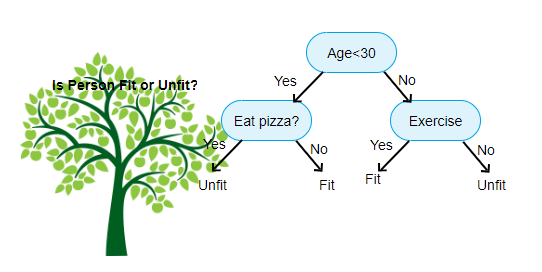
$M$ 個のクラスに分割したとして、
$$\text{Information gain} = \text{Entropy}(S) - \left\{\text{Entropy}(S_1) + \cdots + \text{Entropy}(S_M)\right\}$$が最大になるように条件を設定する。
In [8]:
from kerasy.ML.tree import DecisionTreeClassifier
In [9]:
N=150; K=3
In [10]:
data = np.concatenate([
    np.random.RandomState(0).multivariate_normal(mean=[0, 0], cov=np.eye(2), size=int(N/3)),
    np.random.RandomState(0).multivariate_normal(mean=[1, 5], cov=np.eye(2), size=int(N/3)),
    np.random.RandomState(0).multivariate_normal(mean=[3, 2], cov=np.eye(2), size=int(N/3)),
])
x,y = data.T
In [11]:
cls = np.concatenate([
    np.full(shape=int(N/3), fill_value=0),
    np.full(shape=int(N/3), fill_value=1),
    np.full(shape=int(N/3), fill_value=2),
])
In [12]:
xmin,ymin = np.min(data, axis=0)
xmax,ymax = np.max(data, axis=0)
Xs,Ys = np.meshgrid(np.linspace(xmin, xmax, 100), np.linspace(ymin, ymax, 100))
XYs = np.c_[Xs.ravel(),Ys.ravel()]
In [13]:
model = DecisionTreeClassifier(criterion="gini", max_depth=3, random_state=0)
model.fit(data, cls)
predictions = model.predict(data)
In [14]:
# Decision Tree
Zs = model.predict(XYs).reshape(Xs.shape)
In [15]:
fig = plt.figure(figsize=(18,4))
for i, seed in enumerate([0,1,5]):
    ax = fig.add_subplot(1,3,i+1)
    model = DecisionTreeClassifier(criterion="gini", max_depth=3, random_state=seed)
    model.fit(data, cls)
    predictions = model.predict(data)
    Zs = model.predict(XYs).reshape(Xs.shape)
    ax.scatter(x,y,c=predictions, s=50)
    ax.pcolor(Xs,Ys,Zs,alpha=0.2)
    ax.set_title(f"Decision Tree seed={seed}"), ax.set_xlim(xmin,xmax), ax.set_ylim(ymin,ymax)
    ax.set_xticks([]), ax.set_yticks([])
plt.tight_layout()
plt.show()

Support Vector Machine(SVM)
$$f(\mathbf{x}) = \mathbf{w}\cdot\mathbf{x} + \mathbf{b} = \mathbf{0}$$
$\|\mathbf{w}\|$ を決定するためには、黄色の線上にある点(support vector)のみ寄与。SVMの重要なところは、通常
$$\mathrm{Error}_{\text{世の中全体}}>\mathrm{Error}_{\text{見たことのある世界}}$$であるが、発明者 Vapnic が
$$\mathrm{Error}_{\text{世の中全体}}\leq\mathrm{Error}_{\text{見たことのある世界}} + \alpha$$を証明してしまった。なお、$\alpha$ も $\|\mathbf{w}\|$ の最小化で最小化できるため、$\|\mathbf{w}\|$ の最小化をひたすら頑張るだけで良い。
※ 実装はここ
アンサンブル学習
| 名前 | 説明 | 強学習器 |
|---|---|---|
| bagging | トレーニングデータをランダムにサンプリングして学習器 $f^b(\mathbf{x}),(b=1,2,\ldots,B)$ を作る。 | $$f(\mathbf{x}) = \frac{1}{B}\sum_b^Bf^b(\mathbf{x})$$ |
| Random Forest (RF) | 決定木 $f^r(\mathbf{x}),(r=1,2,\ldots,R)$ をランダムに作る。木がたくさんあるので森(forest)になる。 | $$f(\mathbf{x}) = \frac{1}{R}\sum_r^Rf^r(\mathbf{x})$$ |
| boosting | 弱学習器 $f^t(\mathbf{x})$ の精度に応じた重み付き多数決を行う。なお、$\alpha$ の決め方はadaboostやXGboostなど様々ある。 | $$f(\mathbf{x}) = \frac{1}{T}\sum_t^T\alpha^tf^t(\mathbf{x})$$ |
Neural Network
パーセプトロン
$\mathbf{w}$ を法線と考えると、超平面のあっちとこっちを判定しているだけ=SVMと同じ。 perceptronの学習アルゴリズムは、下記の流れで収束することが知られている。
- 重み(法線)ベクトルをランダムに設定
- 2クラス $0,1$ があったとして、training dataから順に取り出して、$y$ を出力してみる(平面のどちら側か)
- 合っていたら何もしない。間違っていたら $$ \begin{cases} \mathbf{w}\longleftarrow\mathbf{w} +\rho \mathbf{x} & (\text{クラス1を0と誤判定した時})\\ \mathbf{w}\longleftarrow\mathbf{w} -\rho \mathbf{x} & (\text{クラス0を1と誤判定した時}) \end{cases}$$
- 2,3を全てのtraining dataに対して行う。
- 全てのtraining dataに対して正解が規定回数に達したら終了。それ以外の場合、2に戻る。
# Pythonでプログラム化すると以下。
while True:
    n_true=0
    for x,c in zip(data,cls):
        if   c==1 and sum(w*x)<0 : w+=rho*x
        elif c==0 and sum(w*x)>=0: w-=rho*x
        else: n_true+=1
    if n_true>N*true_rate: break
In [16]:
n_cls0 = 30; n_cls1 = 40
N = n_cls0 + n_cls1
In [17]:
w = np.random.RandomState(0).uniform(size=2) # Initialization.
rho = 1e-3 # step size.
true_rate = 0.9
In [18]:
# train_x
data = np.concatenate([
    np.random.RandomState(0).multivariate_normal(mean=[2,4], cov=np.eye(2), size=n_cls0),
    np.random.RandomState(0).multivariate_normal(mean=[3,1], cov=np.eye(2), size=n_cls1),
])
X1,X2 = data.T
# train_t
cls = np.concatenate([
    np.zeros(shape=(n_cls0), dtype=int),
    np.ones(shape=(n_cls1),  dtype=int)
])
In [19]:
while True:
    n_true=0
    for x,c in zip(data,cls):
        if   c==1 and sum(w*x)<0 : w+=rho*x
        elif c==0 and sum(w*x)>=0: w-=rho*x
        else: n_true+=1
    if n_true>N*true_rate: break
In [20]:
X = np.linspace(min(X1),max(X2),1000)
Y = (-w[0]/w[1])*X
In [21]:
plt.scatter(X1,X2,c=cls)
plt.plot(X,Y,color="red")
plt.xlabel("$x_1$", fontsize=18), plt.ylabel("$x_2$", fontsize=18)
plt.show()

In [ ]: