teilab.statistics module

This submodule contains various functions and classes that are useful for statistical testing.

Instructions

Statistical hypothesis testing

Statistical hypothesis testing is required to determine if expression levels (gProcessedSignal s) have changed between samples with siRNA and those without siRNA.

A statistical hypothesis test is a method of statistical inference. An alternative hypothesis is proposed for the probability distribution of the data. The comparison of the two models is deemed statistically significant if, according to a threshold probability—the significance level ( \(\alpha\) ) — the data would be unlikely to occur if the null hypothesis were true. The pre-chosen level of significance is the maximal allowed “false positive rate”. One wants to control the risk of incorrectly rejecting a true null hypothesis.

The process of distinguishing between the null hypothesis and the alternative hypothesis is aided by considering two conceptual types of errors.

1. The first type of error occurs when the null hypothesis is wrongly rejected. (type 1 error)

2. The second type of error occurs when the null hypothesis is wrongly not rejected. (type 2 error)

Hypothesis tests based on statistical significance are another way of expressing confidence intervals (more precisely, confidence sets). In other words, every hypothesis test based on significance can be obtained via a confidence interval, and every confidence interval can be obtained via a hypothesis test based on significance. 1

1

Mathematical Statistics and Data Analysis (3rd ed.)

See also

Statistical_hypothesis_testing

Various alternative hypotheses can be handled by changing the value of A

In this submodules, you can test each null (alternative) hypothesis by changing the value of alternative

Terminology	alternative	Alternative Hypothesis	Rejection Region
right-tailed	"greater"	\(H_a:\sigma^2_1 > \sigma^2_2\)	\(\mathbf{F}\geq F_{\alpha}\)
left-tailed	"less"	\(H_a:\sigma^2_1 < \sigma^2_2\)	\(\mathbf{F}\leq F_{1−\alpha}\)
two-tailed	"two-sided"	\(H_a:\sigma^2_1 \neq \sigma^2_2\)	\(\mathbf{F}\leq F_{1−\alpha∕2}\) or \(\mathbf{F}\geq F_{\alpha∕2}\)

Follow the chart below to select the test.

Distributions

• gamma-distribution

• f-distribution

• t-distribution

gamma-distribution

The gamma function is defined as

\[\Gamma(z) = \int_0^\infty t^{z-1} e^{-t} dt\]

for \(\Re(z) > 0\) and is extended to the rest of the complex plane by analytic continuation.

The gamma function is often referred to as the generalized factorial since \(\Gamma(n + 1) = n!\) for natural numbers \(n\). More generally it satisfies the recurrence relation \(\Gamma(z + 1) = z \cdot \Gamma(z)\) for complex \(z\), which, combined with the fact that \(\Gamma(1) = 1\), implies the above identity for \(z = n\).

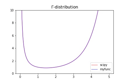
>>> import numpy as np
>>> import matplotlib.pyplot as plt
>>> from scipy.special import gamma
>>> from scipy.integrate import quad
>>> def gamma_pdf(x):
...     return quad(func=lambda x,z:np.power(x, z-1)*np.exp(-x), a=0, b=np.inf, args=(x))[0]
>>> x = np.linspace(1e-2, 5, 100)
>>> fig, ax = plt.subplots(figsize=(6, 4))
>>> ax.plot(x, gamma(x), color="red", alpha=0.5, label="scipy")
>>> ax.plot(x, np.vectorize(gamma_pdf)(x), color="blue", alpha=0.5, label="myfunc")
>>> ax.set_title(fr"$\Gamma$-distribution", fontsize=14)
>>> ax.legend()
>>> ax.set_ylim(0, 10)
>>> fig.savefig("statistics.distributions.gamma.jpg")

Results

f-distribution

The probability density function for f is:

\[f(x, df_1, df_2) = \frac{df_2^{df_2/2} df_1^{df_1/2} x^{df_1 / 2-1}}{(df_2+df_1 x)^{(df_1+df_2)/2}B(df_1/2, df_2/2)}\]

for \(x > 0\).

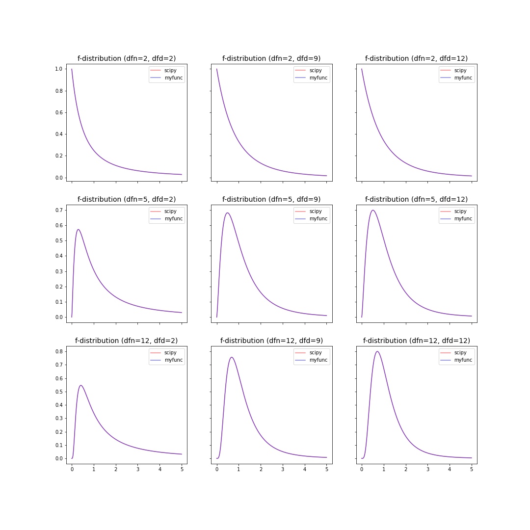
>>> import numpy as np
>>> import matplotlib.pyplot as plt
>>> from scipy import stats
>>> from scipy.special import beta
>>> def f_pdf(x,dfn,dfd):
...     return (dfd**(dfd/2) * dfn**(dfn/2) * x**(dfn/2-1)) / ((dfd+dfn*x)**((dfn+dfd)/2) * beta(dfn/2, dfd/2))
>>> dfns = [2,5,12]; dfds = [2,9,12]
>>> x = np.linspace(0.001, 5, 1000)
>>> fig, axes = plt.subplots(nrows=len(dfns), ncols=len(dfds), sharex=True, sharey="row", figsize=(5*len(dfns), 5*len(dfds)))
>>> for axes_row, dfn in zip(axes, dfns):
...     for ax, dfd in zip(axes_row, dfds):
...         ax.plot(x, stats.f.pdf(x, dfn=dfn, dfd=dfd), color="red", alpha=0.5, label="scipy")
...         ax.plot(x, f_pdf(x, dfn=dfn,dfd=dfd), color="blue", alpha=0.5, label="myfunc")
...         ax.set_title(f"f-distribution (dfn={dfn}, dfd={dfd})", fontsize=14)
...         ax.legend()
>>> fig.show()

Results

t-distribution

The probability density function for t is:

\[f(x, \nu) = \frac{\Gamma((\nu+1)/2)}{\sqrt{\pi \nu} \Gamma(\nu/2)}(1+x^2/\nu)^{-(\nu+1)/2}\]

where \(x\) is a real number and the degrees of freedom parameter \(\nu\) satisfies \(\nu > 0\).

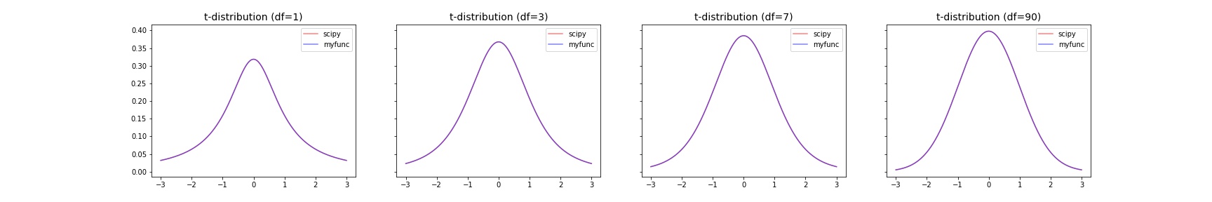
>>> import numpy as np
>>> import matplotlib.pyplot as plt
>>> from scipy import stats
>>> from scipy.special import gamma
>>> def t_pdf(x,df):
...     return gamma((df+1)/2) / (np.sqrt(np.pi*df)*gamma(df/2)) * (1+x**2/df)**(-(df+1)/2)
>>> x = np.linspace(-3, 3, 1000)
>>> dfs = [1,3,7,90]
>>> fig, axes = plt.subplots(nrows=1, ncols=len(dfs), sharey="row", figsize=(6*len(dfs), 4))
>>> for ax,df in zip(axes,dfs):
...     ax.plot(x, stats.t.pdf(x, df=df), color="red", alpha=0.5, label="scipy")
...     ax.plot(x, t_pdf(x, df=df), color="blue", alpha=0.5, label="myfunc")
...     ax.set_title(f"t-distribution (df={df})", fontsize=14)
...     ax.legend()
>>> fig.show()

Results

Notation

sample means

Let

\[\overline{X}=\frac{1}{n_X}\sum_{i=1}^{n_X}X_{i}\]

be the sample means.

sample variances

Let

\[\begin{split}S_X^2&={\frac{1}{n_X-1}}\sum_{i=1}^{n_X}\left(X_{i}-{\overline{X}}\right)^{2}\\&={\frac{1}{n_X-1}}\left(\sum_{i=1}^{n_X}X_i^2-n_X\overline{X}^2\right)\end{split}\]

be the sample variances.

Python Objects

class teilab.statistics.TestResult(statistic: float, pvalue: float, alpha: float, alternative: str, accepts: Tuple[float, float], distribution: callable, distname: str = '', testname: str = '')

Bases: object

Structure that holds test results.

Parameters

• statistic (float) – Test-specific statistical value.

• pvalue (float) – The probability that an observed difference could have occurred just by random chance.

• alpha (float) – The probability of making the wrong decision when the null hypothesis is true.

• alternative (str) – Defines the alternative hypothesis. Please choose from [ "two-sided", "less", "greater" ]

• accepts (Tuple[float,float]) – Regions that accepts the null hypothesis.

• distribution (callable) – Distribution used during the test.

• distname (str, optional) – The distribution name. Defaults to "".

• testname (str, optional) – The test name. Defaults to "".

does_H0_hold

Does the null hypothesis hold?

Type

bool

plot(x: Optional[nptyping.types._ndarray.NDArray[Any, nptyping.types._object.Object]] = None, ax: Optional[matplotlib.axes._axes.Axes] = None) → matplotlib.axes._axes.Axes

Plot the test result.

Parameters

• x (Optional[NDArray[Any, Number]], optional) – X-axis Values. Defaults to None.

• ax (Optional[Axes], optional) – An instance of Axes. Defaults to None.

Returns

An instance of Axes with test result.

Return type

Axes

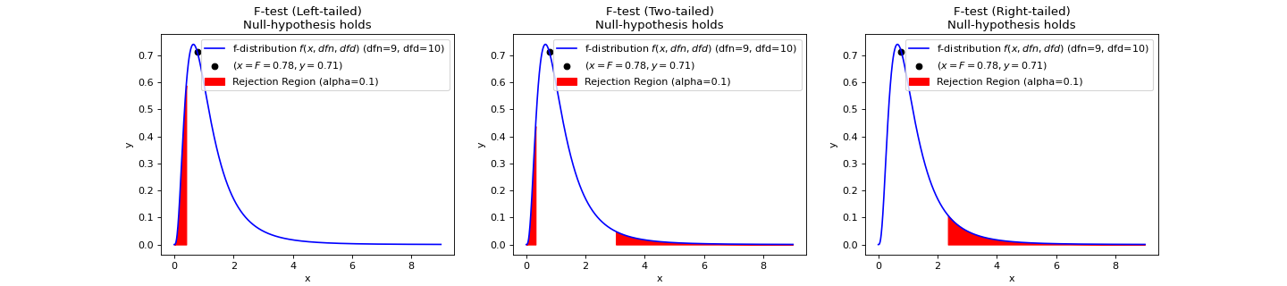
teilab.statistics.f_test(a: nptyping.types._ndarray.NDArray[Any, nptyping.types._object.Object], b: nptyping.types._ndarray.NDArray[Any, nptyping.types._object.Object], alpha: float = 0.05, alternative: str = 'two-sided', plot: bool = False, ax: Optional[matplotlib.axes._axes.Axes] = None) → teilab.statistics.TestResult

F-test for Equality of TWO Variances.

If the two populations are normally distributed and if \(H_0:\sigma^2_1=\sigma^2_2\) is true then under independent sampling \(F\) approximately follows an F-distribution (\(f(x, df_1, df_2)\)) with degrees of freedom \(df_1=n_1−1\) and \(df_2=n_2−1\).

Statistic ( \(F\) )

\[F={\frac {S_{A}^{2}}{S_{B}^{2}}}\]

Parameters

• a (NDArray[Any, Number]) – (Observed) Samples. The arrays must have the same shape.

• b (NDArray[Any, Number]) – (Observed) Samples. The arrays must have the same shape.

• alpha (float) – The probability of making the wrong decision when the null hypothesis is true.

• alternative (str, optional) – Defines the alternative hypothesis. Please choose from [ "two-sided", "less", "greater" ]. Defaults to "two-sided".

• plot (bool, optional) – Whether to plot F-distribution or not. Defaults to False.

• ax (Optional[Axes], optional) – An instance of Axes. The distribution is drawn here when plot is True . Defaults to None.

Returns

Structure that holds F-test results.

Return type

TestResult

Raises

KeyError – When alternative is not selected from [ "two-sided", "less", "greater" ].

>>> import numpy as np
>>> from teilab.utils import subplots_create
>>> from teilab.statistics import f_test
>>> fig, axes = subplots_create(ncols=3, figsize=(18,4), style="matplotlib")
>>> A = np.array([6.3, 8.1, 9.4, 10.4, 8.6, 10.5, 10.2, 10.5, 10.0, 8.8])
>>> B = np.array([4.8, 2.1, 5.1,  2.0, 4.0,  1.0,  3.4,  2.7,  5.1, 1.4, 1.6])
>>> for ax,alternative in zip(axes,["less","two-sided","greater"]):
...     f_test(A, B, alternative=alternative, plot=True, alpha=.1, ax=ax)
>>> fig.show()

See also

F-test

teilab.statistics.student_t_test(a: nptyping.types._ndarray.NDArray[Any, nptyping.types._object.Object], b: nptyping.types._ndarray.NDArray[Any, nptyping.types._object.Object], alpha: float = 0.05, alternative: str = 'two-sided', plot: bool = False, ax: Optional[matplotlib.axes._axes.Axes] = None) → teilab.statistics.TestResult

T-test for Equality of averages of TWO INDEPENDENT samples. (SIMILAR VARIANCES)

Statistic ( \(T\) )

\[T={\frac{\overline{A}-{\overline{B}}}{s_p\cdot {\sqrt {\frac{1}{n_A}+\frac{1}{n_B}}}}}\]

where

\[s_p=\sqrt{\frac {\left(n_A-1\right)s_A^2+\left(n_B-1\right)s_B^2}{n_A+n_B-2}}\]

Parameters

• a (NDArray[Any, Number]) – (Observed) Samples. The arrays must have the same shape.

• b (NDArray[Any, Number]) – (Observed) Samples. The arrays must have the same shape.

• alpha (float) – The probability of making the wrong decision when the null hypothesis is true.

• alternative (str, optional) – Defines the alternative hypothesis. Please choose from [ "two-sided", "less", "greater" ]. Defaults to "two-sided".

• plot (bool, optional) – Whether to plot F-distribution or not. Defaults to False.

• ax (Optional[Axes], optional) – An instance of Axes. The distribution is drawn here when plot is True . Defaults to None.

Returns

Structure that holds student’s T-test results.

Return type

TestResult

Raises

KeyError – When alternative is not selected from [ "two-sided", "less", "greater" ].

>>> import numpy as np
>>> from teilab.utils import subplots_create
>>> from teilab.statistics import student_t_test
>>> fig, axes = subplots_create(ncols=3, figsize=(18,4), style="matplotlib")
>>> A = np.array([6.3, 8.1, 9.4, 10.4, 8.6, 10.5, 10.2, 10.5, 10.0, 8.8])
>>> B = np.array([4.8, 2.1, 5.1,  2.0, 4.0,  1.0,  3.4,  2.7,  5.1, 1.4, 1.6])
>>> for ax,alternative in zip(axes,["less","two-sided","greater"]):
...     student_t_test(A, B, alternative=alternative, plot=True, alpha=.1, ax=ax)
>>> fig.show()

See also

• T-test

• scipy.stats.ttest_ind(A, B, equal_var=True)

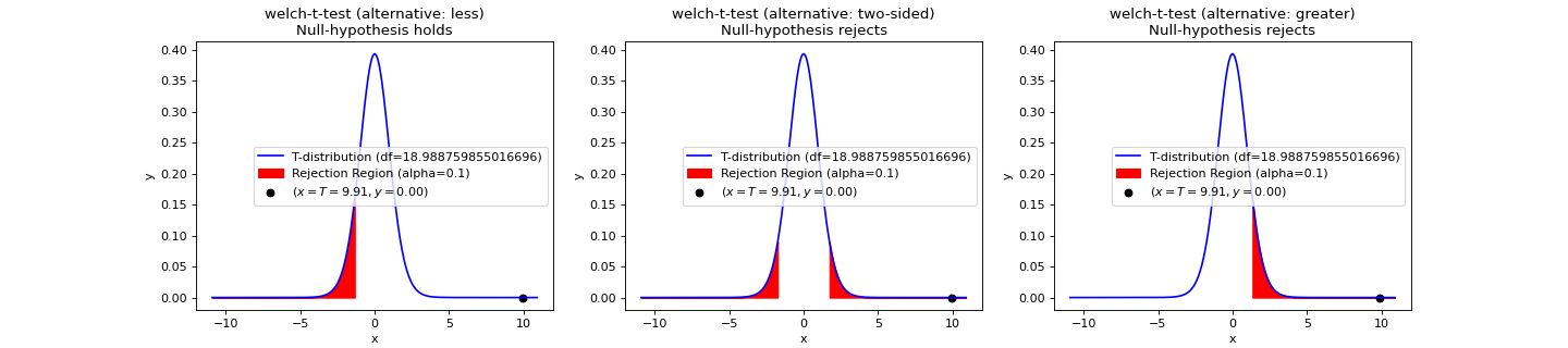
teilab.statistics.welch_t_test(a: nptyping.types._ndarray.NDArray[Any, nptyping.types._object.Object], b: nptyping.types._ndarray.NDArray[Any, nptyping.types._object.Object], alpha: float = 0.05, alternative: str = 'two-sided', plot: bool = False, ax: Optional[matplotlib.axes._axes.Axes] = None) → teilab.statistics.TestResult

T-test for Equality of averages of TWO INDEPENDENT samples. (DIFFERENT VARIANCES)

Statistic ( \(T\) )

\[T=\frac{\Delta\overline {X}}{s_{\Delta\overline{X}}}=\frac{\overline{X}_1-\overline{X}_2}{\sqrt{{s^2_{\overline{X}_1}}+s^2_{\overline{X}_{2}}}}\]

where

\[s_{{\overline{X}}_{i}}={s_i\over{\sqrt{N_i}}}\]

Parameters

• a (NDArray[Any, Number]) – (Observed) Samples. The arrays must have the same shape.

• b (NDArray[Any, Number]) – (Observed) Samples. The arrays must have the same shape.

• alpha (float) – The probability of making the wrong decision when the null hypothesis is true.

• alternative (str, optional) – Defines the alternative hypothesis. Please choose from [ "two-sided", "less", "greater" ]. Defaults to "two-sided".

• plot (bool, optional) – Whether to plot F-distribution or not. Defaults to False.

• ax (Optional[Axes], optional) – An instance of Axes. The distribution is drawn here when plot is True . Defaults to None.

Returns

Structure that holds welch’s T-test results.

Return type

TestResult

Raises

KeyError – When alternative is not selected from [ "two-sided", "less", "greater" ].

>>> import numpy as np
>>> from teilab.utils import subplots_create
>>> from teilab.statistics import welch_t_test
>>> fig, axes = subplots_create(ncols=3, figsize=(18,4), style="matplotlib")
>>> A = np.array([6.3, 8.1, 9.4, 10.4, 8.6, 10.5, 10.2, 10.5, 10.0, 8.8])
>>> B = np.array([4.8, 2.1, 5.1,  2.0, 4.0,  1.0,  3.4,  2.7,  5.1, 1.4, 1.6])
>>> for ax,alternative in zip(axes,["less","two-sided","greater"]):
...     welch_t_test(A, B, alternative=alternative, plot=True, alpha=.1, ax=ax)
>>> fig.show()

See also

• T-test

• Welch’s_t-test

• scipy.stats.ttest_ind(A, B, equal_var=False)

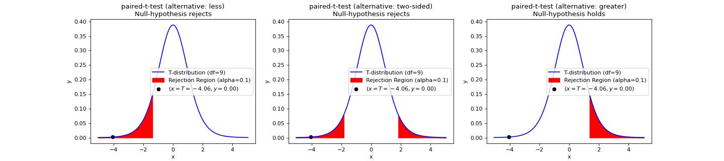
teilab.statistics.paired_t_test(a: nptyping.types._ndarray.NDArray[Any, nptyping.types._object.Object], b: nptyping.types._ndarray.NDArray[Any, nptyping.types._object.Object], alpha: float = 0.05, alternative: str = 'two-sided', plot: bool = False, ax: Optional[matplotlib.axes._axes.Axes] = None) → teilab.statistics.TestResult

T-test for Equality of averages of TWO RELATED samples.

Statistic ( \(T\) )

\[T=\frac{\overline{D}}{S_D/\sqrt{N}}\]

where \(D\) is the sample differences ( \(D=A-B\) ), \(N\) is the sample length ( \(N=\mathrm{len}(A)=\mathrm{len}(B)\))

Parameters

• a (NDArray[Any, Number]) – (Observed) Samples. The arrays must have the same shape.

• b (NDArray[Any, Number]) – (Observed) Samples. The arrays must have the same shape.

• alpha (float) – The probability of making the wrong decision when the null hypothesis is true.

• alternative (str, optional) – Defines the alternative hypothesis. Please choose from [ "two-sided", "less", "greater" ]. Defaults to "two-sided".

• plot (bool, optional) – Whether to plot F-distribution or not. Defaults to False.

• ax (Optional[Axes], optional) – An instance of Axes. The distribution is drawn here when plot is True . Defaults to None.

Returns

Structure that holds paired T-test results.

Return type

TestResult

Raises

• TypeError – When the arrays a and b have the different shapes.

• KeyError – When alternative is not selected from [ "two-sided", "less", "greater" ].

>>> import numpy as np
>>> from teilab.utils import subplots_create
>>> from teilab.statistics import paired_t_test
>>> fig, axes = subplots_create(ncols=3, figsize=(18,4), style="matplotlib")
>>> A = np.array([0.7, -1.6, -0.2, -1.2, -0.1, 3.4, 3.7, 0.8, 0.0, 2.0])
>>> B = np.array([1.9,  0.8,  1.1,  0.1, -0.1, 4.4, 5.5, 1.6, 4.6, 3.4])
>>> for ax,alternative in zip(axes,["less","two-sided","greater"]):
...     paired_t_test(A, B, alternative=alternative, plot=True, alpha=.1, ax=ax)
>>> fig.show()

See also

• T-test

• scipy.stats.ttest_ind(A, B)

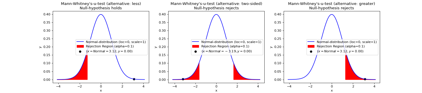
teilab.statistics.mann_whitney_u_test(a: nptyping.types._ndarray.NDArray[Any, nptyping.types._object.Object], b: nptyping.types._ndarray.NDArray[Any, nptyping.types._object.Object], alpha: float = 0.05, alternative: str = 'two-sided', use_continuity: bool = True, plot: bool = False, ax: Optional[matplotlib.axes._axes.Axes] = None) → teilab.statistics.TestResult

NON-PARAMETRIC-test for Equality of averages of TWO INDEPENDENT samples.

Mann–Whitney U test is used as significance

Statistic ( \(U\) )

Let \(A_{1},\ldots, A_{n}\) be an i.i.d. sample from \(A\), and \(B_{1},\ldots ,B_{m}\) be an i.i.d. sample from \(B\), and both samples independent of each other. The corresponding Mann-Whitney \(U\) statistic is defined as:

\[U=\sum_{i=1}^{n_A}\sum_{j=1}^{n_B}S(A_{i},B_{j})\]

with

\[\begin{split}S(A,B)={\begin{cases}1,&{\text{if }}B<A,\\{\tfrac {1}{2}},&{\text{if }}B=A,\\0,&{\text{if }}B>A.\end{cases}}\end{split}\]

In direct method, for each observation in sample a, the sum of the number of observations in sample b for which a smaller value was obtained is the \(U_A\) .

In other method, \(U_A\) is given by:

\[U_A=R_A-\frac{n_A(n_A+1)}{2}\]

where \(n_A\) is the sample size for sample a, and \(R_A\) is the sum of the ranks in sample a because \(\frac{n_A(n_A+1)}{2}\) is the sum of all the ranks of a within sample a.

Knowing that \(R_A+R_B=N(N+1)/2\) and \(N=n_A+n_B\), we find that the sum is

\[\begin{split}U_A + U_B &= \left(R_A - \frac{n_A(n_A+1)}{2}\right) + \left(R_B - \frac{n_B(n_B+1)}{2}\right) \\ &= \underbrace{\left(R_A + R_B\right)}_{(N)(N+1)/2} - \frac{1}{2}\left(n_A(n_A+1) + n_B(n_B+1)\right)\\ &= n_An_B.\end{split}\]

For large ( \(>20\) ) samples, \(U\) is approximately normally distributed. In this case, the standardized value

\[z={\frac {U-m_{U}}{\sigma _{U}}}\]

where \(m_U\) and \(\sigma_U\) are the mean and standard deviation of \(U\), is approximately a standard normal deviate whose significance can be checked in tables of the normal distribution. \(m_U\) and \(\sigma_U\) are given by

\[\begin{split}m_U={\frac {n_An_B}{2}},\ \text{and} \\ \sigma _{U}={\sqrt {\frac{n_An_B(n_A+n_B+1)}{12}}}.\end{split}\]

The formula for the standard deviation is more complicated in the presence of tied ranks. If there are ties in ranks, \(\sigma\) should be corrected as follows:

\[\sigma _{\text{corr}}={\sqrt {\frac{n_An_B}{12}\left((N+1)-\sum_{i=1}^k\frac{t_i^3-t_i}{N(N-1)}\right)}}\]

where \(N=n_A+n_B, t_i\) is the number of subjects sharing rank \(i\), and \(k\) is the number of (distinct) ranks.

Warning

How to calculate the statistic value is different from scipy.

Parameters

• a (NDArray[Any, Number]) – (Observed) Samples. The arrays must have the same shape.

• b (NDArray[Any, Number]) – (Observed) Samples. The arrays must have the same shape.

• alpha (float) – The probability of making the wrong decision when the null hypothesis is true.

• alternative (str, optional) – Defines the alternative hypothesis. Please choose from [ "two-sided", "less", "greater" ]. Defaults to "two-sided".

• use_continuity (bool, optional) – Whether a continuity correction ( 1/2. ) should be taken into account. Default is True .

• plot (bool, optional) – Whether to plot F-distribution or not. Defaults to False.

• ax (Optional[Axes], optional) – An instance of Axes. The distribution is drawn here when plot is True . Defaults to None.

Returns

Structure that holds Mann-Whitney’s U-tesst results.

Return type

TestResult

Raises

• KeyError – When alternative is not selected from [ "two-sided", "less", "greater" ].

• ValueError – When all numbers are identical in mannwhitneyu.

>>> import numpy as np
>>> from teilab.utils import subplots_create
>>> from teilab.statistics import mann_whitney_u_test
>>> fig, axes = subplots_create(ncols=3, figsize=(18,4), style="matplotlib")
>>> A = np.array([1.83, 1.50, 1.62, 2.48, 1.68, 1.88, 1.55, 3.06, 1.30, 2.01, 3.11])
>>> B = np.array([0.88, 0.65, 0.60, 1.05, 1.06, 1.29, 1.06, 2.14, 1.29])
>>> for ax,alternative in zip(axes,["less","two-sided","greater"]):
...     mann_whitney_u_test(A, B, alternative=alternative, plot=True, alpha=.1, ax=ax)
>>> fig.show()

See also

• Mann-Whitney_U_test

• On a Test of Whether one of Two Random Variables is Stochastically Larger than the Other

• scipy.stats.mannwhitneyu(A, B)

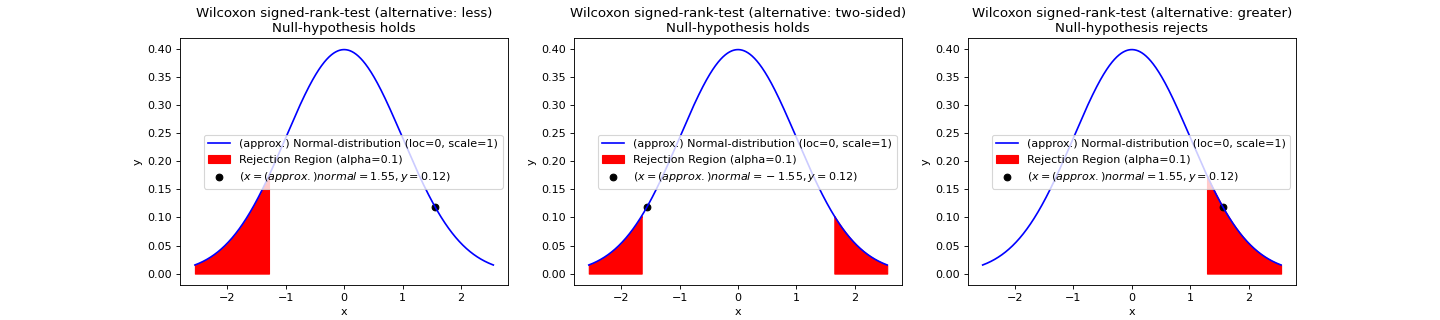
teilab.statistics.wilcoxon_test(a: nptyping.types._ndarray.NDArray[Any, nptyping.types._object.Object], b: nptyping.types._ndarray.NDArray[Any, nptyping.types._object.Object], alpha: float = 0.05, alternative: str = 'two-sided', mode: str = 'auto', plot: bool = False, ax: Optional[matplotlib.axes._axes.Axes] = None) → teilab.statistics.TestResult

NON-PARAMETRIC-test for Equality of representative values (medians) of TWO PAIRED samples.

This function is about the Wilcoxon signed-rank test which tests whether the distribution of the differences a - b is symmetric about zero. It is a non-parametric version of the paired_t_test.

Note

Wilcoxon signed-rank test is different from Wilcoxon rank sum test which is equivalent to the student_t_test or welch_t_test in the parametric test.

Statistic ( \(W\) )

Let \(N\) be the sample size, i.e., the number of pairs (\(A=a_i,\ldots,a_N, B=b_i,\ldots,b_N\)).

1. Exclude pairs with \(|a_i-b_i|=0\). Let \(N_r\) be the reduced sample size.

2. Order the remaining \(N_r\) pairs acoording to the absolute difference (\(|a_i-b_i|\)).

3. Rank the pairs. Ties receive a rank equal to the average og the ranks they span (assign_rank(a-b, method="average")). Let \(R_i\) denote the rank.

4. Calculate the test statistic \(W\) (the sum of the signed ranks)

\[\begin{split}W_{+}&=\sum_{i=1}^{N_r}\left[\operatorname{sgn}(a_i-b_i)\cdot R_{i}\right],\\ W_{-}&=\sum_{i=1}^{N_r}\left[-\operatorname{sgn}(a_i-b_i)\cdot R_{i}\right].\end{split}\]

5. From the above, use \(W\) that matches the alternative hypothesis.

\[\begin{split}W=\begin{cases} \mathrm{min}\left(W_{+},W_{-}\right),&\text{if alternative hypothesis is "two-tailed"},\\ W_{+},&\text{otherwise.} \end{cases}\end{split}\]

6. As \(N_r\) increases, the sampling distribution of \(W\) converges to a normal distribution. Thus,

   1. For \(N_r\geq25\), a z-score can be calculated as

   \[Z = \frac{\left|W-\frac{N_r(N_r+1)}{4}\right|}{\sqrt{\frac{N_r(N_r+1)(2N_r+1)}{24}}}\]

   2. For \(N_r<25\) the exact distribution needs to be used.

Parameters

• a (NDArray[Any, Number]) – (Observed) Samples. The arrays must have the same shape.

• b (NDArray[Any, Number]) – (Observed) Samples. The arrays must have the same shape.

• alpha (float) – The probability of making the wrong decision when the null hypothesis is true.

• alternative (str, optional) – Defines the alternative hypothesis. Please choose from [ "two-sided", "less", "greater" ]. Defaults to "two-sided".

• mode (str, optional) – Method to calculate the p-value. Please choose from [ "auto", "exact", "approx" ]. Default is “auto”.

• plot (bool, optional) – Whether to plot F-distribution or not. Defaults to False.

• ax (Optional[Axes], optional) – An instance of Axes. The distribution is drawn here when plot is True . Defaults to None.

Returns

Structure that holds wilcoxon-test results.

Return type

TestResult

Raises

• TypeError – When the arrays a and b have the different shapes.

• KeyError – When alternative is not selected from [ "two-sided", "less", "greater" ].

• ValueError – When all pairs are identical, or try to calculate "exact" p-value with the sample size larger than 25.

>>> import numpy as np
>>> from teilab.utils import subplots_create
>>> from teilab.statistics import wilcoxon_test
>>> fig, axes = subplots_create(ncols=3, figsize=(18,4), style="matplotlib")
>>> rnd = np.random.RandomState(0)
>>> A,B = rnd.random_sample(size=(2,30))
>>> for ax,alternative in zip(axes,["less","two-sided","greater"]):
...     wilcoxon_test(A, B, alternative=alternative, plot=True, alpha=.1, ax=ax)
>>> fig.show()

See also

• https://docs.scipy.org/doc/scipy/reference/generated/scipy.stats.kruskal.html#scipy.stats.kruskal

• https://docs.scipy.org/doc/scipy/reference/generated/scipy.stats.mannwhitneyu.html#scipy.stats.mannwhitneyu

• scipy.stats.wilcoxon(A, B, correction=False, alternative=”two-sided”)

• Wilcoxon_signed-rank_test

teilab.statistics.anova() → teilab.statistics.TestResult

teilab.statistics.friedman_test() → teilab.statistics.TestResult

teilab.statistics.kruskal_wallis_test() → teilab.statistics.TestResult