teilab.normalizations module

This submodule contains various functions and classes that are useful for normalization.

Instructions

Differential gene expression can be an outcome of true biological variability or experimental artifacts. Normalization techniques have been used to minimize the effect of experimental artifacts on differential gene expression analysis.

Robust Multichip Analysis (RMA)

In microarray analysis, many algorithms have been proposed, but the most widely used one (de facto standard) is Robust Multichip Analysis (RMA) , where the signal value of each spot ( RawData ) is processed and normalized according to the following flow. ( 1) Background Subtraction, 2) Normalization Between Samples and 3) Summarization )

1. Background Subtraction

In Background Subtraction, we assume that the observed signal intensity is a combnation of the actual signal intensity and the background signal intensity (derived from Non-specific Hybridization), and aim to eliminate the influence of the latter one.

In the general method, we make assumptions such as

• Actual signal intensity distribution is an exponential distribution.

• Background signal intensity distribution is a normal distribution.

Then, by optimizing the parameters to best represent the phenomenon, the background intensity distribution is calculated and subtracted.

2. Normalization Between Samples

Here, we perform normalization “between” samples. What can be said from the results of a “single sample” microarray experiment are very limited, and we should compare with other (treatment sample, control group, etc.) experimental results. Howevet, bias due to experimental operation and equipment characteristics is inevitable, and if you just compare them as they are, you will misinterpret them.

For example, if you want to characterize the changes in global gene expression in the livers of H1/siRNAinsulin-CMV/hIDE transgenic (Tg) mice in response to the reduced bioavailability of insulin 1, and the expression level of each RNA in Tg mice was generally lower than that of non-Tg mice, you may mistakenly conclude that almost all of the RNAs were down-regulated respectively by reduced bioavailability of insulin.

1

Microarray analysis of insulin-regulated gene expression in the liver: the use of transgenic mice co-expressing insulin-siRNA and human IDE as an animal model

Therefore, it is necessary to reduce the influence of the bias. There are numerous proposals for normalizing unbalanced data between samples ( This review paper summarizes 23 normalization methods developed for unbalanced transcriptome data), but each method makes some assumptions in data, so it is important to choose the correct normalization method for each experimental results.

We will introduce two majour methods.

Note

1. Percentile

2. Quantile

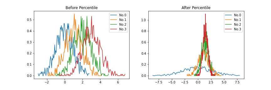
1. Percentile

This method is a constant adjustoment and the most straightforward.

1. Calculate the x%tile for each distribution.

2. Average them.

3. Divide each distribution by its x%tile and multiply by averaged value.

Example

Defined as percentile in this package.

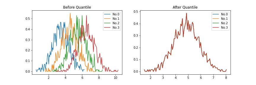
2. Quantile

Quantile Normalization is a technique for making all distributions identical in statistical properties. It was introduced as “quantile standardization” (in Analysis of Data from Viral DNA Microchips ) and then renamed as “quantile normalization” (in A comparison of normalization methods for high density oligonucleotide array data based on variance and bias )

To quantile normalize the all distributions,

1. Sort each distribution.

2. Average the data in the same rank.

3. Replace the value of each rank with the averaged value.

Warning

This method can be used when the assumption that “the intensity distribution of gene expression in each sample is almost the same” holds.

Example

Defined as quantile in this package.

3. Summarization

https://github.com/scipy/scipy/blob/v1.6.3/scipy/signal/signaltools.py#L3384-L3467

Python Objects

teilab.normalizations.percentile(data: nptyping.types._ndarray.NDArray[Any, Any, nptyping.types._object.Object], percent: numbers.Number = 75) → nptyping.types._ndarray.NDArray[Any, Any, nptyping.types._object.Object]

Perform Percentile Normalization.

Parameters

• data (NDArray[(Any,Any),Number]) – Input data. Shape = ( n_samples, n_features )

• percent (Number, optional) – Which percentile value to normalize. Defaults to 75.

Returns

percentiled data. Shape = ( n_samples, n_features )

Return type

NDArray[(Any,Any),Number]

Raises

ValueError – When percent tiles contain negative values.

Examples

>>> import matplotlib.pyplot as plt
>>> from teilab.normalizations import percentile
>>> from teilab.plot.matplotlib import densityplot
>>> n_samples, n_features = (4, 1000)
>>> data = np.random.RandomState(0).normal(loc=np.expand_dims(np.arange(n_samples), axis=1),  size=(n_samples,n_features))
>>> data_percentiled = percentile(data=data, percent=75)
>>> fig, axes = plt.subplots(ncols=2, nrows=1, figsize=(12,4))
>>> ax = densityplot(data=data, title="Before Percentile", ax=axes[0])
>>> ax = densityplot(data=data_percentiled, title="After Percentile", ax=axes[1])

Results

teilab.normalizations.quantile(data: nptyping.types._ndarray.NDArray[Any, Any, nptyping.types._object.Object]) → nptyping.types._ndarray.NDArray[Any, Any, nptyping.types._object.Object]

Perform Quantile Normalization.

Parameters

data (NDArray[(Any,Any),Number]) – Input data. Shape = ( n_samples, n_features )

Returns

percentiled data. Shape = ( n_samples, n_features )

Return type

NDArray[(Any,Any),Number]

Raises

ValueError – When data contains negative values.

Examples

>>> import matplotlib.pyplot as plt
>>> from teilab.normalizations import quantile
>>> from teilab.plot.matplotlib import densityplot
>>> n_samples, n_features = (4, 1000)
>>> data = np.random.RandomState(0).normal(loc=np.expand_dims(np.arange(n_samples), axis=1), size=(n_samples,n_features), ) + 3.5
>>> data_quantiled = quantile(data=data)
>>> fig, axes = plt.subplots(ncols=2, nrows=1, figsize=(12,4))
>>> ax = densityplot(data=data, title="Before Quantile", ax=axes[0])
>>> ax = densityplot(data=data_quantiled, title="After Quantile", ax=axes[1])

Results

teilab.normalizations.median_polish(data: nptyping.types._ndarray.NDArray[Any, Any, nptyping.types._object.Object], labels: nptyping.types._ndarray.NDArray[Any, Any], rtol: float = 1e-05, atol: float = 1e-08) → nptyping.types._ndarray.NDArray[Any, Any, nptyping.types._object.Object]

Median Polish

Parameters

• data (NDArray[(Any,Any),Number]) – Input data. Shape = ( n_samples, n_features )

• labels (NDArray[(Any),Any]) – Label (ex. GeneName, or SystematicName )

• rtol (float) – The relative tolerance parameter. Defaults to 1e-05

• atol (float) – The absolute tolerance parameter. Defaults to 1e-08

Raises

TypeError – When data.shape[1] is not the same as len(labels)

Returns

Median Polished Data.

Return type

NDArray[(Any,Any),Number]

Examples

>>> from teilab.normalizations import median_polish
>>> data = np.asarray([
...     [16.1, 14.6, 19.6, 13.6, 13.6, 13.6],
...     [ 9.0, 18.4,  6.7, 11.1,  6.7,  9.0],
...     [22.4, 13.6, 22.4,  6.7,  9.0,  3.0],
>>> ], dtype=float).T
>>> n_samples, n_features = data.shape
>>> # This means that "All spots (features) are for the same gene."
>>> labels = np.zeros(shape=n_features, dtype=np.uint8)
>>> median_polish(data, labels=labels)
array([[16.1 , 11.25, 13.3 ],
       [16.4 , 11.55, 13.6 ],
       [19.6 , 14.75, 16.8 ],
       [13.6 ,  8.75, 10.8 ],
       [11.8 ,  6.95,  9.  ],
       [13.6 ,  8.75, 10.8 ]])

Todo

Speed-UP using joblib, multiprocessing, Cython, etc.

teilab.normalizations.median_polish_group_wise(data: pandas.core.generic.NDFrame, rtol: float = 1e-05, atol: float = 1e-08) → pandas.core.generic.NDFrame

Apply Median polish group-wise.

Parameters

• data (NDFrame) – Input data. Shape = ( n_samples, n_features )

• rtol (float, optional) – [description]. Defaults to 1e-05.

• atol (float, optional) – [description]. Defaults to 1e-08.

Returns

Median Polished Data.

Return type

NDFrame

Examples

>>> from teilab.normalizations import median_polish_group_wise
>>> data = pd.DataFrame(data=[
...     ["vimentin", 16.1, 14.6, 19.6, 13.6, 13.6, 13.6],
...     ["vimentin",  9.0, 18.4,  6.7, 11.1,  6.7,  9.0],
...     ["vimentin", 22.4, 13.6, 22.4,  6.7,  9.0,  3.0],
>>> ], columns=["GeneName"]+[f"Samle.{i}" for i in range(6)])
>>> data.groupby("GeneName").apply(func=median_polish_group_wise).values
array([[16.1 , 16.4 , 19.6 , 13.6 , 11.8 , 13.6 ],
       [11.25, 11.55, 14.75,  8.75,  6.95,  8.75],
       [13.3 , 13.6 , 16.8 , 10.8 ,  9.  , 10.8 ]])
>>> # If you want to see the progress, use tqdm.
>>> from tqdm import tqdm
>>> tqdm.pandas()
>>> data.groupby("GeneName").progress_apply(func=median_polish_group_wise).values